Regression Analysis Explained: Types, Methods, and Predictions
Master predicting numbers - from house prices to stock forecasts
Read 15 min
Regression Supervised Learning Machine Learning Linear Regression Prediction Algorithms
Every time Zillow estimates your home's value, Tesla predicts battery range, or Netflix forecasts server load, regression algorithms are working behind the scenes. Regression is the foundation of predictive analytics, powering everything from financial forecasting (stock prices, revenue projections) to scientific modeling (climate predictions, drug dosage) to business optimization (inventory planning, pricing strategies). The core task: learn from historical data to predict future numerical values.
Abbreviations Used in This Article
MLMachine Learning
SVMSupport Vector Machine
MSEMean Squared Error
RMSERoot Mean Squared Error
MAEMean Absolute Error
ROIReturn on Investment
FAQFrequently Asked Questions
Key Terms Explained
This tutorial uses several technical terms. Hover over highlighted terms like CoefficientCoefficientA number that tells you how much each feature affects the prediction. Larger coefficients mean that feature has more influence on the outcome.Example:If square footage has coefficient 0.5, adding 100 sq ft increases predicted price by $50,000., RegularizationRegularizationA technique to prevent models from becoming too complex and overfitting. It adds a penalty for using too many features or making coefficients too large.Example:Like adding a speed limit to prevent your model from memorizing training data instead of learning patterns., or OverfittingOverfittingWhen a model memorizes the training data too well, including noise and outliers, so it performs poorly on new data.Example:A student who memorizes exam answers but can't apply concepts to new problems. to see simple explanations. These tooltips provide beginner-friendly definitions without breaking your reading flow.
What Makes This Tutorial Different
This is your entry point to regression analysis. We'll explain the fundamentals using intuitive examples, introduce the most common algorithms briefly, and show you when to use each approach. Dedicated pages for individual methods (coming soon) will cover implementation details and advanced techniques.
What You'll Master in This Guide
01
What is Regression? - Understanding how machines predict continuous values from data
02
How Regression Works - The step-by-step process from data to predictions
03
Regression vs Classification - When to predict numbers vs categories
04
Types of Regression - Simple, multiple, polynomial, and non-linear regression
05
Common Regression Methods - Overview of 7 popular regression algorithms
06
How to Choose a Method - Simple decision framework for selecting algorithms
07
Real-World Applications - Where regression is used in industry
08
Common Challenges - Top pitfalls and how to avoid them
09
Your Learning Journey - Roadmap through regression methods
10
Frequently Asked Questions - Quick answers to common regression questions
What is Regression: Predicting Continuous Values in Machine Learning
Imagine you're a real estate agent trying to price a house that just came on the market. You look at similar houses that recently sold: a 2,000 sq ft house sold for $350,000, a 2,500 sq ft house for $425,000, a 3,000 sq ft house for $500,000. You notice a pattern: roughly $150 per square foot, plus adjustments for bedrooms, location, and age. Now a client asks: "What should we price our 2,750 sq ft house?" You estimate around $460,000 based on the pattern you learned. That's regression - finding mathematical relationships in data to predict continuous values.
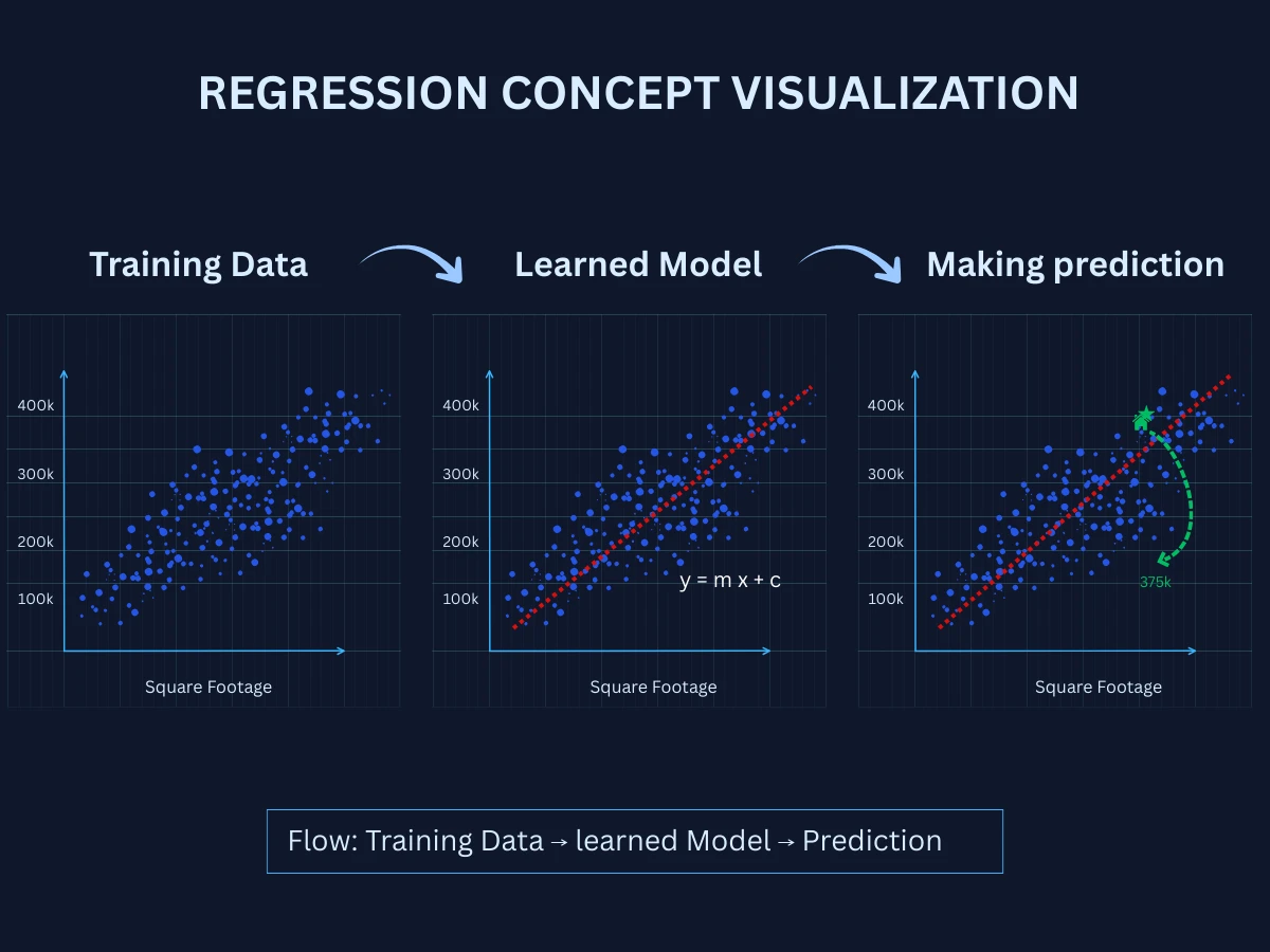
In machine learning, regression is a supervised learning task where the algorithm learns to predict continuous numerical outputs from input features. Unlike classification, which predicts discrete categories (spam/not spam, cat/dog), regression predicts values on a continuous scale (house price: $327,450, temperature: 72.3 degrees, probability: 0.847). The algorithm discovers mathematical relationships between inputs and outputs by analyzing training examples, then uses those relationships to make predictions on new data.
Regression Concept - From training data to predictions: the model learns a mathematical relationship and uses it to estimate values for new unseen data
How Regression Works: Finding Patterns to Predict Numerical Outcomes
Regression follows a systematic process from collecting historical data to making accurate predictions. Understanding this workflow is essential for building effective regression systems. Here's the step-by-step process:
1
Collect Labeled Training Data
Gather examples with known input-output pairs. For house price prediction, collect data on homes with features (square footage, bedrooms, location) and their actual sale prices. For sales forecasting, gather historical sales data with relevant factors (advertising spend, season, promotions).
2
Extract and Select Features
Identify measurable characteristics that influence the target value. House price features might include size, age, location, number of rooms. Sales features might include marketing budget, time of year, economic indicators. Good features have strong correlation with the target.
3
Train the Regression Model
The algorithm learns the mathematical relationship between features and the target value. It fits a line, curve, or complex function that best predicts the output from inputs. The model minimizes prediction errors on training data.
4
Make Predictions on New Data
Apply the trained model to new, unseen examples. Given features of a house not in the training set, predict its price. Given this month's marketing spend, predict expected sales. The model uses learned patterns to estimate continuous values.
5
Evaluate and Improve
Measure how far predictions are from actual values using metrics like RMSE or MAE. Analyze errors to identify patterns. Improve by adding better features, trying different algorithms, collecting more data, or adjusting model complexity.
The key insight: regression algorithms learn mathematical functions that map inputs to outputs. Simple problems might use a straight line (linear regression). Complex problems might need curves (polynomial regression) or sophisticated functions (neural networks). The goal is always the same: minimize the difference between predicted values and actual values on training data, then generalize that learning to make accurate predictions on new data.
Regression vs Classification: When to Use Each
Both regression and classification are supervised learning tasks, but they predict fundamentally different outputs. Understanding this difference helps you frame problems correctly and choose appropriate algorithms.
Regression vs Classification: Core Differences
Aspect
Regression
Classification
Output Type
Continuous numerical values
Discrete categories/classes
Goal
Predict a number on a continuous scale
Assign data to predefined groups
Example Output
House price: $325,000, Temperature: 72.5 degrees
'spam' or 'not spam', 'cat', 'dog', or 'bird'
Model Fit
Fits a line/curve through data points
Creates boundaries separating classes
Evaluation Metrics
MSE, RMSE, MAE, R-squared
Accuracy, precision, recall, F1-score
Common Algorithms
Linear regression, polynomial regression, random forests
Logistic regression, decision trees, SVM
Use Case Examples
Stock price prediction, sales forecasting, temperature prediction
Email spam detection, medical diagnosis, image recognition
Prediction Range
Any value within reasonable bounds (can be infinite)
Fixed set of predefined categories
Source: Comparison based on standard supervised learning taxonomy
Quick Decision Rule
Ask yourself: "Is the answer a number or a category?" If you're predicting a value that can fall anywhere on a scale (price, temperature, count, probability as a decimal), use regression. If you're choosing between fixed labels from a predefined set (approved/rejected, cat/dog, high/medium/low risk), use classification.
Types of Regression Problems: Linear, Polynomial, and Regularized Models
Regression problems vary based on the number of input features, the relationship shape, and the complexity of the underlying patterns. Understanding these distinctions helps you select appropriate modeling approaches.
Four Main Types of Regression
Type
Number of Features
Relationship Shape
Example Problem
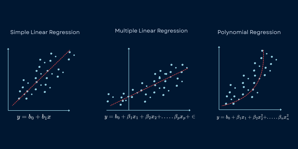
Simple Linear Regression
1 input feature
Straight line relationship
Predict house price from square footage only Predict exam score from hours studied Predict crop yield from rainfall
Multiple Linear Regression
2+ input features
Linear combination of features
Predict house price from size, age, location, bedrooms Predict sales from advertising, price, season Predict car price from mileage, age, brand, condition
Polynomial Regression
1+ features
Curved, non-linear relationship
Predict stopping distance from speed (quadratic) Predict enzyme activity vs temperature (optimal peak) Predict learning progress over time (diminishing returns)
Non-Linear Regression
1+ features
Complex, arbitrary relationships
Predict stock prices with technical indicators Predict customer lifetime value with behavior patterns Predict energy consumption with weather and time patterns
Source: Standard regression taxonomy from statistical learning literature
Real-World Example: Predicting Delivery Time
A delivery company might use: Simple regression - estimate time from distance alone. Multiple regression - add factors like traffic, weather, package weight. Polynomial regression - account for non-linear effects (traffic impact increases exponentially with distance). Non-linear regression - use neural networks to capture complex patterns like rush hour, weather interactions, and seasonal variations.
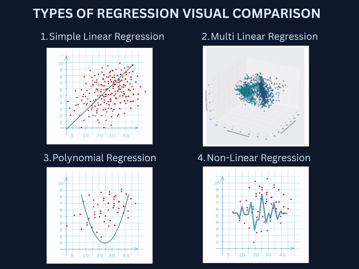
Types of Regression - Simple linear, multiple linear, polynomial, and non-linear regression each model different relationships between inputs and outputs
Common Regression Algorithms: Linear, Ridge, Lasso, and Neural Networks
There are many regression algorithms, each with different strengths and ideal use cases. Here are the seven most common methods you'll encounter. Each will have a dedicated tutorial page for in-depth learning - this section provides a quick introduction to help you understand when to use each approach.
1. Linear Regression: Predicting Continuous Values with a Straight Line
Linear regression is the foundation of all regression methods. It assumes a straight-line relationship between inputs and output, finding the best-fit line that minimizes prediction errors. Think of it as drawing the line that gets closest to all your data points. It's fast, interpretable, and works surprisingly well for many real-world problems despite its simplicity.
Best for: Linear relationships, when you need interpretability, quick baseline models
Strengths: Very fast training, works with small datasets, easy to interpret coefficients, predictions have confidence intervals
Limitations: Assumes linear relationship, sensitive to outliers, struggles with complex patterns
This example trains a linear regression model on California housing data to predict median house values. The model achieves R-squared of 0.576, meaning it explains 57.6% of price variance. The coefficients show feature importance - for example, median income (0.437) has strong positive impact on price.
2. Polynomial Regression: Capturing Non-Linear Relationships in Data
Polynomial regression extends linear regression to handle curved relationships by using polynomial terms (x-squared, x-cubed, etc.). It can fit U-shapes, S-curves, and other non-linear patterns while maintaining the simplicity of linear methods. You're still fitting a line, but in a transformed feature space where curves become straight lines.
Best for: Non-linear relationships with clear curve patterns, small to medium datasets
Strengths: Handles curves and peaks, still interpretable, works with existing linear regression tools
Limitations: Prone to overfitting with high degrees, extrapolation can be unreliable, manual degree selection
Common uses: Growth curves, optimal point prediction (temperature vs yield), physics modeling
Polynomial Regression with Degree ComparisonPython
This example demonstrates how polynomial degree affects model fit. The data has a true quadratic (degree 2) relationship. Degree 1 (linear) underfits with R-squared of 0.882. Degree 2 captures the pattern perfectly (0.989). Higher degrees (3, 5) show marginal gains but risk overfitting on noise.
3. Ridge Regression: L2 Regularization to Prevent Overfitting
Ridge regression is linear regression with a penalty on large coefficient values. This L2 Regularization (Ridge)L2 Regularization (Ridge)A regularization method that shrinks all coefficients toward zero but keeps them all in the model. Prevents any single feature from having too much influence.Example:Reduces the impact of correlated features like "square footage" and "number of rooms" without removing either. prevents overfitting by constraining the model complexity. It's particularly valuable when you have many FeatureFeatureAn input variable or characteristic that your model uses to make predictions. Also called an attribute or predictor.Example:For house price prediction: square footage, number of bedrooms, location are all features. or MulticollinearityMulticollinearityWhen two or more features in your model are highly correlated with each other, making it hard to determine which one actually affects the prediction.Example:Both "square footage" and "number of rooms" increase together, so the model can't tell which one really drives house prices. (correlated features). The algorithm trades a bit of training accuracy for better generalization to new data.
Best for: Many features, correlated features (multicollinearity), preventing overfitting
Strengths: Reduces overfitting, handles correlated features well, more stable than plain linear regression
Limitations: Doesn't eliminate features (keeps all with small weights), requires tuning regularization strength
Common uses: High-dimensional data, economic modeling, genomics, any regression with many predictors
10# Compare different regularization strengths (alpha values)
11alphas = [0.01, 0.1, 1.0, 10.0, 100.0]
12for alpha in alphas:
13 ridge = Ridge(alpha=alpha)
14 ridge.fit(X_train, y_train)
15 train_score = ridge.score(X_train, y_train)
16 test_score = ridge.score(X_test, y_test)
17 print(f"Alpha {alpha:5.2f}: Train R2={train_score:.3f}, Test R2={test_score:.3f}")
18
19# Output:
20# Alpha 0.01: Train R2=0.606, Test R2=0.576 (weak regularization)
21# Alpha 0.10: Train R2=0.606, Test R2=0.576 (optimal balance)
22# Alpha 1.00: Train R2=0.606, Test R2=0.576 (still good)
23# Alpha 10.00: Train R2=0.604, Test R2=0.574 (stronger penalty)
24# Alpha 100.0: Train R2=0.582, Test R2=0.555 (too much - underfitting)
Ridge regression adds an L2 penalty to prevent overfitting. The alpha parameter controls regularization strength. Low alpha (0.01-1.0) maintains performance while reducing overfitting. High alpha (100) penalizes coefficients too much, causing underfitting (test R-squared drops to 0.555). Alpha=0.1-1.0 provides optimal balance.
4. Lasso Regression: L1 Regularization with Automatic Feature Selection
Lasso regression applies L1 Regularization (Lasso)L1 Regularization (Lasso)A regularization method that can reduce some coefficients to exactly zero, effectively removing unimportant features from the model.Example:Automatically identifies that "house color" doesn't affect price and removes it from the model., which not only prevents overfitting but also performs automatic feature selection by driving some coefficients to exactly zero. This makes models simpler and more interpretable by identifying which features actually matter. It's like ridge regression, but with the superpower of eliminating irrelevant features entirely.
Best for: Feature selection, sparse solutions, when many features are irrelevant
Lasso performs automatic feature selection by driving some coefficients to exactly zero. With alpha=0.1, it eliminates AveRooms entirely and nearly eliminates AveOccup, identifying them as less important. The top predictors are MedInc (median income) and location features (Latitude, Longitude). This creates a simpler, more interpretable model.
5. Elastic Net Regression: Combining Ridge and Lasso Regularization
Elastic Net combines the best of ridge and lasso by using both L1 and L2 regularization. It gets the stability of ridge with the feature selection of lasso. This makes it the go-to choice when you have many correlated features and want both regularization and automatic feature selection. Think of it as the versatile middle ground between ridge and lasso.
Best for: Correlated features with automatic selection needed, general-purpose regularization
Strengths: Combines ridge stability with lasso selection, handles correlated features better than lasso alone
Limitations: Two hyperparameters to tune instead of one, slightly more complex
Common uses: General regression with many features, when both ridge and lasso seem applicable
Elastic Net combines L1 (Lasso) and L2 (Ridge) regularization. The l1_ratio parameter controls the mix: 0=pure ridge, 1=pure lasso, 0.5=balanced. With l1_ratio=0.5, it performs feature selection like Lasso while maintaining Ridge's stability with correlated features. All three achieve similar R-squared (0.575-0.576).
6. Decision Tree and Random Forest Regression: Non-Linear Prediction
Decision trees make predictions by splitting data based on feature values, creating a tree of decisions that leads to predicted values. Random forests combine hundreds of trees, averaging their predictions for better accuracy and reduced overfitting. They handle non-linear relationships automatically without assuming any specific function form, making them extremely versatile for complex patterns.
Best for: Non-linear relationships, mixed data types, when you want high accuracy without much tuning
Random forests combine hundreds of decision trees for superior accuracy. A single tree achieves R-squared of 0.616, while the random forest reaches 0.802 - the best performance yet! Random forests automatically capture non-linear relationships and feature interactions. The feature importance shows median income (0.523) is the dominant predictor.
7. Neural Networks for Regression: Deep Learning for Complex Predictions
Neural networks can learn arbitrarily complex relationships between inputs and outputs through layers of interconnected nodes. For regression, they're particularly powerful with high-dimensional data (images, sequences, text) or when patterns are too complex for traditional methods. They require more data and computation but can achieve state-of-the-art accuracy on challenging problems.
Best for: Very large datasets, high-dimensional inputs (images, sequences), extremely complex patterns
Strengths: Handles any complexity, automatic feature learning, state-of-the-art accuracy on hard problems
Limitations: Requires lots of data and compute, black box (hard to interpret), many hyperparameters to tune
Common uses: Image-based prediction (house price from photos), time series forecasting, scientific simulations
Neural Network Regression with Deep LearningPython
1from sklearn.neural_network import MLPRegressor
2from sklearn.preprocessing import StandardScaler
3
4# Neural networks require feature scaling
5scaler = StandardScaler()
6X_train_scaled = scaler.fit_transform(X_train)
7X_test_scaled = scaler.transform(X_test)
8
9# Train neural network with 2 hidden layers
10nn_model = MLPRegressor(
11 hidden_layer_sizes=(100, 50), # 2 layers: 100 neurons, then 50
Neural networks with 2 hidden layers (100 and 50 neurons) achieve R-squared of 0.798, nearly matching random forest performance. The network requires feature scaling and more training time (127 iterations), but can learn complex non-linear patterns automatically. For this tabular data, random forests (0.802) slightly edge out neural networks, but NNs excel with images or sequences.
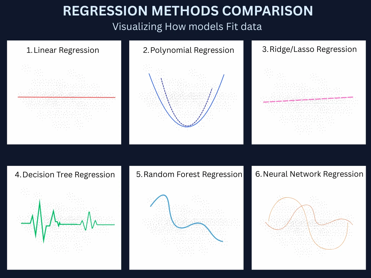
Regression Methods Comparison - Each method fits the same data differently, from simple straight lines to complex curves, making them suited to different problem types
Quick Comparison: When to Use Each Method
Algorithm
Complexity
Interpretability
Training Speed
Best Use Case
Linear Regression
Very simple
Very high
Very fast
Linear relationships, baselines
Polynomial Regression
Simple
High
Fast
Curved relationships with known degree
Ridge Regression
Simple
High
Fast
Many correlated features, prevent overfitting
Lasso Regression
Simple
Very high
Fast
Feature selection, sparse solutions
Elastic Net
Simple
High
Fast
Combines ridge and lasso benefits
Random Forests
High
Medium
Medium
Complex non-linear patterns, high accuracy
Neural Networks
Very high
Very low
Very slow
Images, sequences, extremely complex patterns
Source: Comparison based on standard algorithm characteristics and use cases
How to Choose a Regression Algorithm: Dataset Size, Complexity, and Accuracy
With so many regression algorithms available, how do you choose? Here's a practical decision framework based on your data characteristics and requirements:
Start Simple with Linear Regression: Always begin with basic linear regression. It's fast, interpretable, and often works surprisingly well. If R-squared is > 0.7 and residuals look random, you might be done. This baseline also helps you understand feature importance.
Check for Non-Linearity: Plot predictions vs actual values. If you see clear curved patterns in residuals, try polynomial regression (for simple curves) or random forests (for complex patterns). Don't use linear methods when relationships are obviously non-linear.
Address Overfitting if Present: If training error is much lower than test error, you're overfitting. Try ridge regression (keeps all features), lasso (eliminates features), or elastic net (best of both). Random forests also reduce overfitting through averaging.
Consider Dataset Size: Small dataset (< 1,000 examples)? Stick with linear methods or small random forests. Medium (1,000-100,000)? Any method works. Large (> 100,000)? Consider random forests or neural networks for maximum accuracy.
Evaluate Feature Count: Many features (> 50)? Use ridge, lasso, or elastic net to handle high dimensionality. Need to know which features matter? Use lasso for automatic selection. Very high dimensions (> 1,000 features)? Dimensionality reduction first.
Balance Interpretability vs Accuracy: Need to explain predictions to stakeholders? Use linear, ridge, lasso, or decision trees. Interpretability not critical? Random forests or neural networks typically achieve higher accuracy.
Test Multiple Approaches: Try 2-3 promising methods on your data using cross-validation. Compare R-squared, RMSE, and MAE. The best algorithm depends on your specific dataset - empirical testing beats theoretical assumptions.
The Bias-Variance Tradeoff
Simple models (linear regression) have high bias (underfitting risk) but low variance (consistent predictions). Complex models (neural networks) have low bias but high variance (overfitting risk). The sweet spot depends on your data complexity and size. Start simple, then increase complexity only when simpler models fail.
Real-World Regression Applications: Finance, Healthcare, and Engineering
Regression powers critical predictions across industries. Understanding where and how it's used helps you recognize opportunities to apply these techniques in your own work.
Demand, competitor prices, inventory, time, customer segment
Optimal price point
Healthcare
Dosage optimization
Patient weight, age, kidney function, drug interactions
Optimal drug dosage (mg)
Manufacturing
Yield prediction
Process parameters (temperature, pressure), raw material quality
Production yield percentage
Energy
Demand forecasting
Historical usage, weather, time of day/year, economic activity
Energy consumption (kWh)
Transportation
Delivery time estimation
Distance, traffic, weather, time of day, package weight
Estimated delivery time (minutes)
Marketing
Ad spend optimization
Ad spend by channel, creative quality, targeting, seasonality
Expected ROI or conversions
Agriculture
Crop yield prediction
Rainfall, temperature, soil quality, fertilizer, planting date
Bushels per acre
Source: Common industry applications of regression algorithms
Netflix: Revenue Forecasting at Scale
Netflix uses regression extensively to forecast subscription revenue, predict content performance, and optimize streaming infrastructure capacity. Their models combine time series regression (historical trends), external factors (economic indicators, seasonality), and content features (genre, talent, marketing spend) to predict viewership and revenue months in advance. This enables data-driven decisions on content investment and infrastructure planning.
Common Regression Challenges: Overfitting, Multicollinearity, and Outliers
Regression comes with unique pitfalls that can lead to poor predictions. Understanding these challenges helps you build more robust models:
Overfitting on Training Data: Model learns noise and peculiarities of training data, achieving low training error but high test error. Especially common with polynomial regression (high degree) or complex models. SOLUTION: Use regularization (ridge, lasso), cross-validation, simpler models, or more training data.
Extrapolation Beyond Training Range: Regression models predict poorly outside the range of training data. A model trained on houses $100K-$500K will give unreliable predictions for $2M mansions. SOLUTION: Collect data across the full range you need to predict, or limit predictions to the training data range.
Multicollinearity (Correlated Features): When input features are highly correlated (house size and number of rooms), coefficient estimates become unstable and hard to interpret. Small data changes cause large coefficient swings. SOLUTION: Use ridge or elastic net regression, remove redundant features, or combine correlated features.
Outliers Skewing Predictions: Regression algorithms (especially linear) are sensitive to outliers. A few extreme values can dramatically shift the fitted line, degrading predictions for typical cases. SOLUTION: Detect and investigate outliers, use robust regression methods, transform features (log scale), or use tree-based methods less sensitive to outliers.
Non-Linear Relationships Treated as Linear: Using linear regression when the true relationship is curved leads to systematic prediction errors. The model underfits, missing important patterns. SOLUTION: Visualize relationships, try polynomial terms, use non-linear methods (random forests, neural networks), or transform features.
Heteroscedasticity (Non-Constant Variance): When prediction errors vary across the range (larger errors for high values), standard error estimates and confidence intervals are unreliable. SOLUTION: Transform target variable (log, square root), use weighted regression, or use models that handle varying variance (quantile regression).
Choosing Wrong Evaluation Metrics: RMSE penalizes large errors heavily (good for avoiding big mistakes), while MAE treats all errors equally (good for average performance). R-squared can be misleading with non-linear data. SOLUTION: Use multiple metrics, understand their implications, choose based on business impact of different error types.
The Extrapolation Trap
Regression models should never be trusted outside their training data range. A classic example: linear regression trained on child growth (ages 0-18) would predict an adult of age 80 to be 15 feet tall. Always visualize training data range and limit predictions accordingly. When you must extrapolate, use domain knowledge and add large uncertainty bounds.
Regression Learning Path: Algorithms and Topics to Study Next
Now that you understand regression fundamentals and common methods, you're ready to explore specific algorithms and implementations. Here's the recommended learning path:
Regression Analysis (this page, 16 min): Core concepts, types of regression, overview of 7 common algorithms, and when to use each
Linear Regression Deep Dive (coming soon, 12 min): Least squares, gradient descent, assumptions, diagnostics, and practical implementation
Regularization Methods (coming soon, 15 min): Ridge, lasso, and elastic net in depth - preventing overfitting and feature selection
Tree-Based Regression (coming soon, 16 min): Decision trees, random forests, gradient boosting for complex patterns
Advanced Regression Techniques (coming soon, 18 min): Time series regression, quantile regression, robust methods, and model diagnostics
After mastering regression methods, explore Model Evaluation Metrics to learn how to properly assess regression performance (RMSE, MAE, R-squared), then move to Overfitting and Underfitting to understand the bias-variance tradeoff in depth.
Frequently Asked Questions
01What's the difference between regression and classification?
Regression predicts continuous numerical values (house price: $327,500, temperature: 72.3 degrees). Classification predicts discrete categories (spam/not spam, cat/dog/bird). Use regression when the output is a number on a scale. Use classification when the output is a label from a fixed set of options. Both are supervised learning, but they handle fundamentally different output types.
02Which regression algorithm should I start with?
Always start with simple linear regression. It's fast, interpretable, and works surprisingly well for many problems. If it performs poorly (low R-squared, patterned residuals), try polynomial regression for curved relationships or random forests for complex non-linear patterns. Only use neural networks for very large datasets or high-dimensional inputs like images. Simple methods should always be your baseline.
03How much training data do I need for regression?
It depends on problem complexity and feature count. As a rule of thumb: at least 10-20x examples per feature for linear methods. A model with 5 features needs 50-100+ examples. Complex methods (random forests, neural networks) need more: 1,000-10,000+ examples minimum. Quality matters more than quantity - clean, representative data beats huge noisy datasets. Use learning curves to determine if more data would help.
04What is R-squared and how do I interpret it?
R-squared measures how well your model explains variance in the target variable, ranging from 0 to 1. R-squared = 0.80 means your model explains 80% of variation in the data. Values > 0.7 are often considered good, but it depends on the field. Don't rely on R-squared alone - also check RMSE, MAE, and residual plots. R-squared can be misleading with non-linear models or when comparing models with different feature counts.
05When should I use ridge vs lasso vs elastic net?
Use ridge when you have many correlated features and want to keep all of them with reduced coefficients (no feature selection). Use lasso when you want automatic feature selection - it drives some coefficients to exactly zero, identifying which features matter. Use elastic net when you want both: feature selection and handling of correlated features. Elastic net is often the safest general-purpose choice for high-dimensional regression.
06Can regression predict categorical values?
No, regression predicts continuous numbers. However, you can predict probabilities (continuous 0-1) and then convert to categories using a threshold. For example, logistic regression (despite the name) is classification that uses regression techniques to predict probability of class membership. If you need to predict categories directly, use classification algorithms instead.
07What are residuals and why do they matter?
Residuals are the differences between predicted and actual values: residual = actual - predicted. They reveal model problems: patterns in residual plots indicate missed non-linearity, heteroscedasticity (changing variance), or other violations of assumptions. Good regression models have residuals that are randomly scattered around zero with constant variance. Always plot residuals vs predictions and vs each feature to diagnose issues.
08How do I handle outliers in regression?
First, investigate outliers - they might be errors (fix/remove) or legitimate extreme cases (keep). Options: (1) Use robust regression methods less sensitive to outliers, (2) Transform features/target with log or square root to reduce outlier impact, (3) Use tree-based methods (random forests) naturally resistant to outliers, (4) Winsorize data (cap extreme values), or (5) Use quantile regression that models different parts of the distribution separately.
Next Steps: Deepening Your Understanding of Regression Analysis
You now understand what regression is, how it works, and the most common methods for predicting continuous values. Your next step depends on your learning goals and project needs.
Your Next Step
Want to master specific algorithms? Start with Linear Regression (coming soon) for a deep dive into the foundational regression method, including least squares, assumptions, and diagnostics. Or explore Classification Methods to complete your supervised learning foundation and understand how to predict categories instead of numbers.
Regression is the workhorse of data science. While deep learning dominates headlines, the vast majority of business value comes from well-executed regression on structured data - forecasting revenue, optimizing pricing, predicting demand, estimating risk. Master linear regression deeply, understand when to add complexity, and you'll solve most real-world prediction problems.