Classification Methods Explained: Types, Algorithms, and When to Use Each

Master predicting categories - from spam detection to medical diagnosis

Read 15 min

Classification Supervised Learning Machine Learning Logistic Regression Decision Trees Algorithms

Every time Gmail filters spam, Netflix recommends a show, or your bank flags a fraudulent transaction, classification algorithms are at work. Classification is the most widely-used supervised learning technique, powering everything from medical diagnosis (cancer detection) to autonomous vehicles (object recognition) to social media (content moderation). The core task: given labeled examples, teach a computer to categorize new data into predefined classes.

Abbreviations Used in This Article

AI Artificial Intelligence

ML Machine Learning

SVM Support Vector Machine

KNN K-Nearest Neighbors

RBF Radial Basis Function

SMOTE Synthetic Minority Over-sampling Technique

FAQ Frequently Asked Questions

What Makes This Tutorial Different

This is your entry point to classification methods. We'll explain the fundamentals using simple examples, introduce the most common algorithms briefly, and show you when to use each approach. Dedicated pages for individual methods (coming soon) will cover implementation details.

What You'll Master in This Guide

What is Classification? - Understanding how machines predict categories from data

How Classification Works - The step-by-step process from data to predictions

Classification vs Regression - When to predict categories vs continuous values

Types of Classification - Binary, multiclass, and multilabel classification explained

Common Classification Methods - Overview of 7 popular classification algorithms

How to Choose a Method - Simple decision framework for selecting algorithms

Real-World Applications - Where classification is used in industry

Common Challenges - Top pitfalls and how to avoid them

Your Learning Journey - Roadmap through classification methods

Frequently Asked Questions - Quick answers to common classification questions

What is Classification: Predicting Categories with Machine Learning

Imagine you work at a hospital emergency room, and patients arrive with various symptoms. Your job is to quickly categorize each patient: Does this person have a heart attack, stroke, panic attack, or indigestion? You make this decision by looking at symptoms (chest pain, blood pressure, age, medical history) and matching them to patterns you've learned from thousands of previous cases. That's classification - using known examples to predict which category new cases belong to.

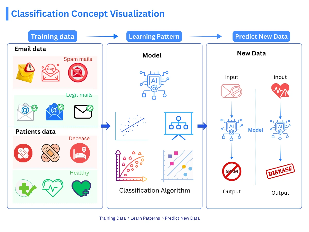
In machine learning, classification is a supervised learning task where the algorithm learns to assign input data to predefined categories (called classes or labels). Unlike regression, which predicts continuous numbers (like house prices or temperatures), classification predicts discrete categories (spam/not spam, cat/dog/bird, high risk/medium risk/low risk). The algorithm learns decision boundaries by studying labeled training examples, then applies those patterns to categorize new, unseen data.

Classification concept visualization showing training data with labeled examples on the left, a model learning decision boundaries in the center, and new unlabeled data being classified on the right — Classification Concept - From labeled training data to predictions: the model learns decision boundaries that separate classes and applies them to new unseen data

How Classification Works: From Training Data to Predictions

Classification follows a systematic process from collecting data to making predictions. Understanding this workflow is essential for building effective classification systems. Here's the step-by-step process:

Collect Labeled Training Data

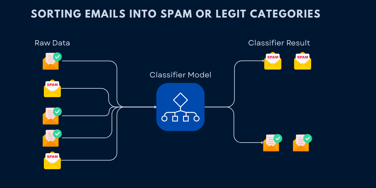
Gather examples where you know the correct category. For email spam detection, this means collecting emails already labeled as 'spam' or 'not spam'. For medical diagnosis, it's patient records with confirmed diagnoses.

Extract Features from Data

Identify measurable characteristics that help distinguish categories. Email features might include word frequency, sender domain, and link count. Medical features might include symptoms, test results, and patient history.

Train the Classification Model

The algorithm analyzes training examples to learn patterns that separate categories. It discovers which feature combinations predict each class. For example, emails with certain keywords and suspicious links tend to be spam.

Make Predictions on New Data

Apply the trained model to new, unlabeled examples. The model examines the features and predicts which category the example belongs to based on learned patterns.

Evaluate and Improve

Test predictions on data the model hasn't seen before. Measure accuracy, identify mistakes, and refine the model by adjusting features, trying different algorithms, or collecting more training data.

The key insight: classification algorithms learn from examples rather than explicit rules. You don't program "if email contains 'free money' then spam" - instead, the algorithm discovers these patterns automatically by analyzing thousands of labeled examples. This makes classification incredibly powerful for complex tasks where rule-based systems would be impractical.

Classification vs Regression: When to Use Each

Both classification and regression are supervised learning tasks, but they predict fundamentally different types of outputs. Understanding this difference is crucial for choosing the right approach for your problem.

Classification vs Regression: Core Differences
Aspect	Classification	Regression
Output Type	Discrete categories/classes	Continuous numerical values
Goal	Assign data to predefined groups	Predict a number on a continuous scale
Example Output	'spam' or 'not spam', 'cat', 'dog', or 'bird'	House price: $325,000, Temperature: 72.5 degrees
Decision Boundary	Creates boundaries separating classes	Fits a line/curve through data points
Evaluation Metrics	Accuracy, precision, recall, F1-score	MSE, RMSE, MAE, R-squared
Common Algorithms	Logistic regression, decision trees, SVM	Linear regression, polynomial regression, ridge
Use Case Examples	Email spam detection, medical diagnosis, image recognition	Stock price prediction, sales forecasting, temperature prediction

Source: Comparison based on standard supervised learning taxonomy

Quick Decision Rule

Ask yourself: "Am I predicting a category or a number?" If the answer is a label from a fixed set of options (spam/not spam, approved/rejected/pending), use classification. If the answer is a numerical value that can fall anywhere on a scale (price, temperature, probability), use regression.

Types of Classification Problems: Binary, Multiclass, and Multilabel

Classification problems come in three main varieties based on how many categories and labels are involved. Understanding these distinctions helps you choose appropriate algorithms and evaluation strategies.

Three Types of Classification
Type	Number of Classes	Labels per Example	Example Problem
Binary Classification	2 classes	1 label (A or B)	Email: spam or not spam Medical test: positive or negative Loan: approved or rejected
Multiclass Classification	3+ classes	1 label (A, B, C, or D...)	Image recognition: cat, dog, bird, or fish News category: sports, politics, tech, or entertainment Plant species: rose, tulip, daisy, or sunflower
Multilabel Classification	Multiple classes	Multiple labels possible	Movie genres: action AND comedy AND sci-fi Article tags: python AND machine-learning AND tutorial Medical conditions: diabetes AND hypertension

Source: Standard classification taxonomy from machine learning literature

Real-World Example: Content Moderation

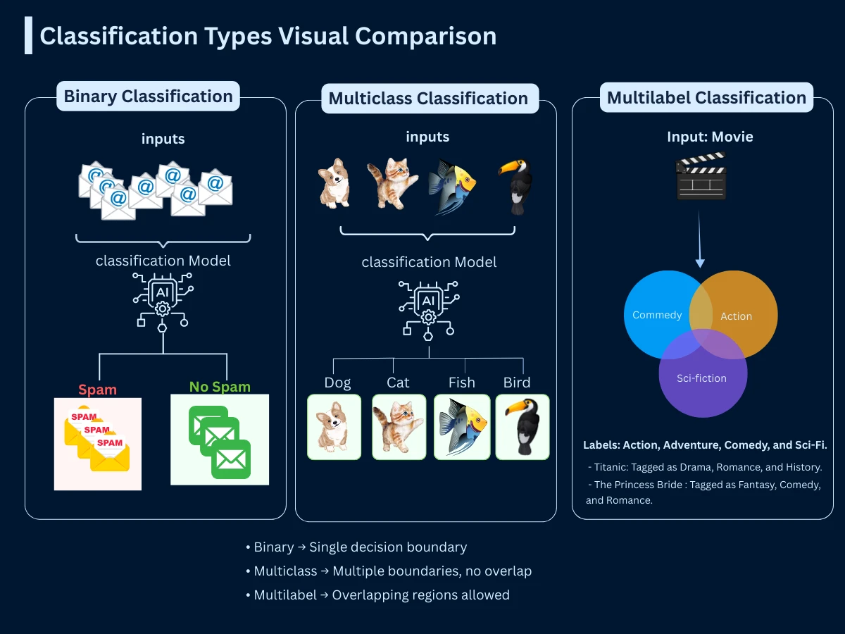
Social media platforms use all three types. Binary: Is this post safe or unsafe? Multiclass: Which category does this violate (hate speech, violence, spam, or misinformation)? Multilabel: This post contains violence AND misinformation AND spam (multiple violations at once).

Three-panel comparison of classification types: binary classification with two separated classes, multiclass with four distinct regions, and multilabel with overlapping categories showing one item belonging to multiple classes — Classification Types - Binary predicts one of two classes, multiclass predicts one of many classes, and multilabel allows multiple simultaneous class assignments

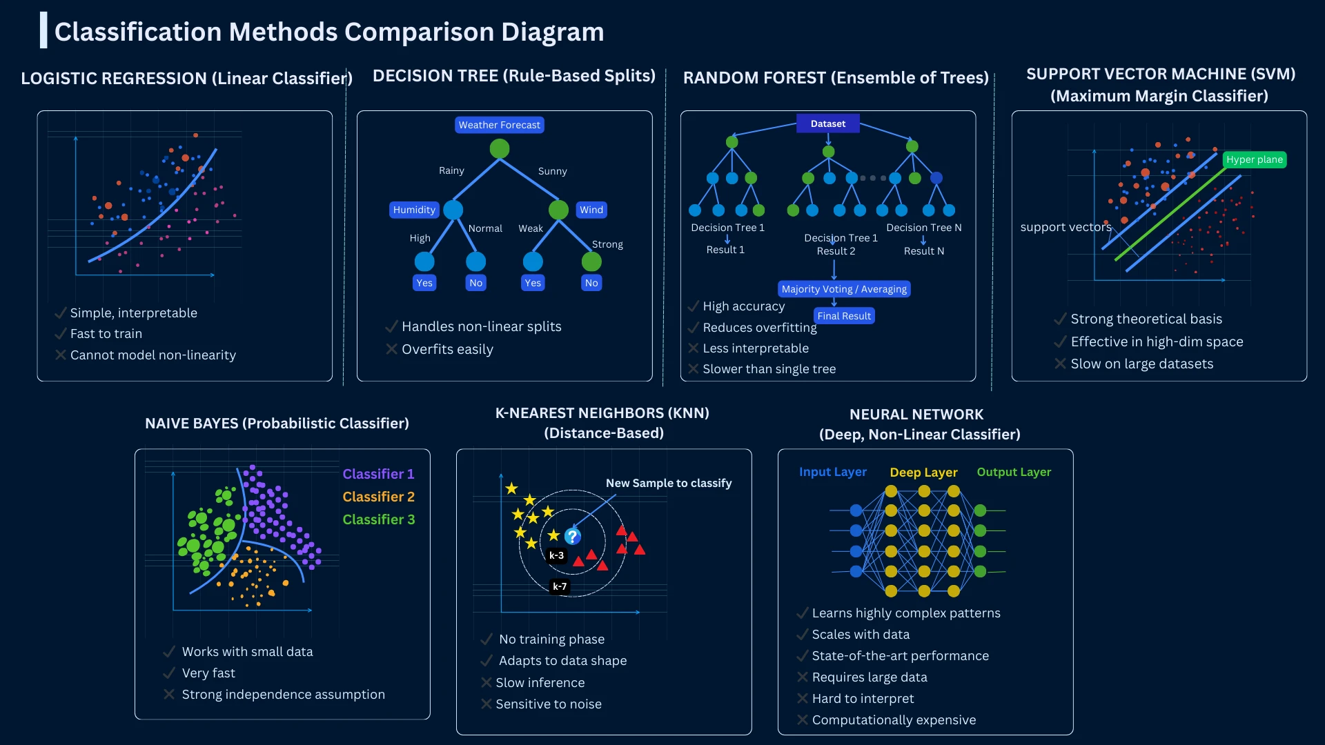
Common Classification Algorithms: Logistic Regression, Trees, and SVM

There are dozens of classification algorithms, each with different strengths and ideal use cases. Here are the seven most common methods you'll encounter. Each will have a dedicated tutorial page for in-depth learning - this section provides a quick introduction to help you understand when to use each approach.

1. Logistic Regression: Probability-Based Binary Classification

Despite its name, logistic regression is used for classification, not regression. It predicts the probability that an example belongs to a particular class, then assigns the class with the highest probability. Think of it as drawing a line (or curve) that separates categories. It's fast, interpretable, and works well when classes are roughly linearly separable.

Best for: Binary classification, when you need probability estimates, interpretable results
Strengths: Fast training, works with small datasets, outputs probabilities, easy to interpret
Limitations: Assumes linear relationship, struggles with complex decision boundaries
Common uses: Email spam detection, credit default prediction, disease diagnosis

Logistic Regression with Scikit-Learn Python


            1
            from sklearn.linear_model import LogisticRegression
          

            2
            from sklearn.model_selection import train_test_split
          

            3
            from sklearn.metrics import accuracy_score, classification_report
          

            4
            from sklearn.datasets import load_wine
          

            5
            
          

            6
            # Load dataset
          

            7
            wine = load_wine()
          

            8
            X, y = wine.data, wine.target
          

            9
            
          

            10
            # Binary classification: Class 0 vs rest
          

            11
            y_binary = (y == 0).astype(int)
          

            12
            
          

            13
            # Split data
          

            14
            X_train, X_test, y_train, y_test = train_test_split(
          

            15
                X, y_binary, test_size=0.2, random_state=42
          

            16
            )
          

            17
            
          

            18
            # Train Logistic Regression
          

            19
            model = LogisticRegression(max_iter=1000)
          

            20
            model.fit(X_train, y_train)
          

            21
            
          

            22
            # Predictions
          

            23
            y_pred = model.predict(X_test)
          

            24
            y_proba = model.predict_proba(X_test)
          

            25
            
          

            26
            # Evaluate
          

            27
            print(f"Accuracy: {accuracy_score(y_test, y_pred):.3f}")
          

            28
            print(f"\nProbability for first sample: {y_proba[0]}")
          

            29
            print(f"Predicted class: {y_pred[0]}")
          

            30
            
          

            31
            # Output:
          

            32
            # Accuracy: 1.000
          

            33
            # Probability for first sample: [0.049 0.951]
          

            34
            # Predicted class: 1

Logistic Regression outputs probabilities for each class (via predict_proba()), then assigns the class with highest probability. The Wine dataset achieves perfect accuracy because Class 0 wines are linearly separable from others.

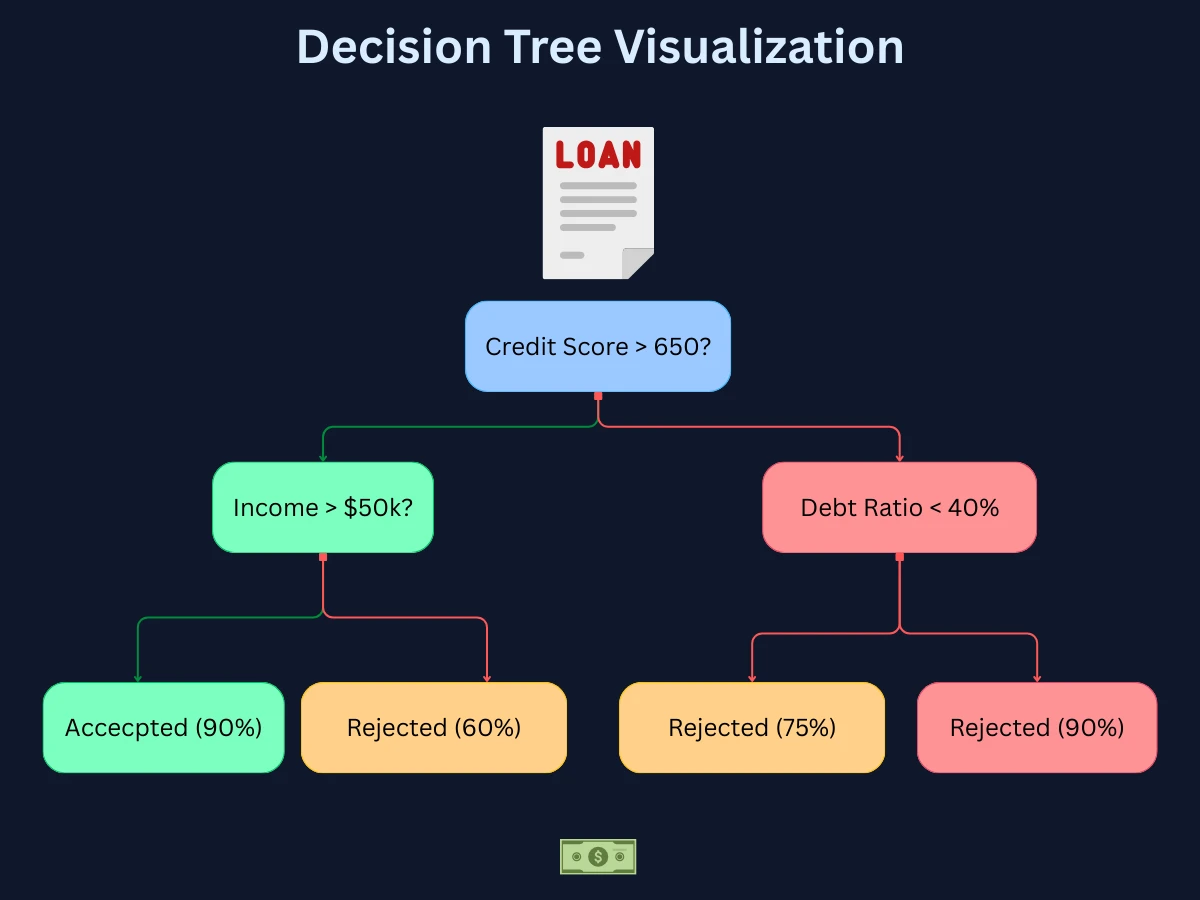
2. Decision Trees: Interpretable Rule-Based Classification

Decision trees make predictions by asking a series of yes/no questions about features, like a flowchart. Each question splits the data based on a feature value until reaching a final classification. They're highly interpretable - you can literally draw the decision-making process - and handle both numerical and categorical data naturally.

Best for: When you need interpretable models, mixed data types, non-linear relationships
Strengths: Easy to visualize and explain, handles missing values, no data scaling needed
Limitations: Prone to overfitting, unstable (small data changes cause big tree changes)
Common uses: Medical diagnosis, customer segmentation, loan approval decisions

Decision Tree with Scikit-Learn Python


            1
            from sklearn.tree import DecisionTreeClassifier
          

            2
            from sklearn.model_selection import train_test_split
          

            3
            from sklearn.metrics import accuracy_score
          

            4
            from sklearn.datasets import load_wine
          

            5
            
          

            6
            # Load dataset
          

            7
            wine = load_wine()
          

            8
            X_train, X_test, y_train, y_test = train_test_split(
          

            9
                wine.data, wine.target, test_size=0.2, random_state=42
          

            10
            )
          

            11
            
          

            12
            # Train Decision Tree
          

            13
            tree = DecisionTreeClassifier(max_depth=3, random_state=42)
          

            14
            tree.fit(X_train, y_train)
          

            15
            
          

            16
            # Predictions
          

            17
            y_pred = tree.predict(X_test)
          

            18
            
          

            19
            # Evaluate
          

            20
            accuracy = accuracy_score(y_test, y_pred)
          

            21
            print(f"Accuracy: {accuracy:.3f}")
          

            22
            
          

            23
            # Feature importance
          

            24
            feature_importance = tree.feature_importances_
          

            25
            top_features = sorted(zip(wine.feature_names, feature_importance),
          

            26
                                 key=lambda x: x[1], reverse=True)[:3]
          

            27
            
          

            28
            print("\nTop 3 Important Features:")
          

            29
            for feature, importance in top_features:
          

            30
                print(f"  {feature}: {importance:.3f}")
          

            31
            
          

            32
            # Output:
          

            33
            # Accuracy: 0.917
          

            34
            # Top 3 Important Features:
          

            35
            #   flavanoids: 0.565
          

            36
            #   proline: 0.245
          

            37
            #   color_intensity: 0.125

Decision trees are highly interpretable - you can see exactly which features the model uses for decisions. The feature_importances_ attribute shows which features contribute most to predictions. Here, flavanoid content is the most important for wine classification.

Decision tree visualization for loan approval showing root node splitting on credit score, with branches for income and debt ratio leading to approved or rejected leaf nodes with confidence percentages and sample decision path highlighted — Decision Tree in Action - A loan approval tree demonstrating how each node splits on a feature threshold, with branches leading to final predictions. The highlighted path shows how a specific applicant's data flows through the tree to reach a decision.

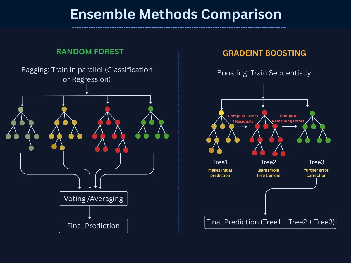
3. Random Forests: Ensemble Method Combining Multiple Decision Trees

Random forests combine hundreds or thousands of decision trees, with each tree voting on the final classification. This ensemble approach reduces overfitting and improves accuracy compared to single decision trees. It's one of the most popular "out-of-the-box" algorithms because it often works well with minimal tuning.

Best for: When you want high accuracy without much tuning, complex datasets
Strengths: Very accurate, reduces overfitting, handles large datasets, feature importance
Limitations: Less interpretable than single trees, slower training and prediction
Common uses: Fraud detection, recommendation systems, gene classification

Random Forest with Scikit-Learn Python


            1
            from sklearn.ensemble import RandomForestClassifier
          

            2
            from sklearn.model_selection import train_test_split
          

            3
            from sklearn.metrics import accuracy_score
          

            4
            from sklearn.datasets import load_wine
          

            5
            
          

            6
            # Load data
          

            7
            wine = load_wine()
          

            8
            X_train, X_test, y_train, y_test = train_test_split(
          

            9
                wine.data, wine.target, test_size=0.2, random_state=42
          

            10
            )
          

            11
            
          

            12
            # Train Random Forest (100 trees)
          

            13
            rf = RandomForestClassifier(n_estimators=100, random_state=42)
          

            14
            rf.fit(X_train, y_train)
          

            15
            
          

            16
            # Predictions
          

            17
            y_pred = rf.predict(X_test)
          

            18
            
          

            19
            # Evaluate
          

            20
            print(f"Accuracy: {accuracy_score(y_test, y_pred):.3f}")
          

            21
            
          

            22
            # Feature importance (averaged across all trees)
          

            23
            importances = rf.feature_importances_
          

            24
            for i, (name, imp) in enumerate(zip(wine.feature_names, importances)):
          

            25
                if imp > 0.1:  # Show only important features
          

            26
                    print(f"{name}: {imp:.3f}")
          

            27
            
          

            28
            # Output:
          

            29
            # Accuracy: 1.000
          

            30
            # proline: 0.180
          

            31
            # flavanoids: 0.153
          

            32
            # color_intensity: 0.145
          

            33
            # od280/od315_of_diluted_wines: 0.128

Random Forests combine 100 decision trees (controlled by n_estimators), with each tree voting on the final prediction. This ensemble approach typically achieves better accuracy than single trees. The feature importances are averaged across all trees.

Two-panel comparison of ensemble methods: Random Forests showing parallel independent trees each voting on the final prediction with majority vote, and Gradient Boosting showing sequential trees where each new tree corrects the previous tree's errors — Ensemble Methods - Random Forests train many trees independently in parallel and combine their votes. Gradient Boosting trains trees sequentially, with each new tree focusing on correcting the errors of previous trees for higher accuracy.

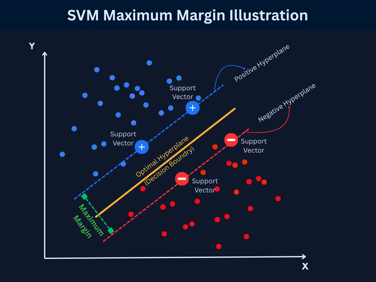
4. Support Vector Machines (SVM): Maximum-Margin Classification

SVM finds the optimal boundary (called a hyperplane) that separates classes with the maximum margin. It's particularly powerful for high-dimensional data and can handle non-linear boundaries using the "kernel trick." While training can be slow, SVMs often achieve excellent accuracy on complex problems.

Best for: High-dimensional data (many features), when you need maximum-margin separation
Strengths: Effective in high dimensions, memory efficient, versatile (via kernels)
Limitations: Slow training on large datasets, requires feature scaling, hard to interpret
Common uses: Text classification, image recognition, bioinformatics

Support Vector Machine with Scikit-Learn Python


            1
            from sklearn.svm import SVC
          

            2
            from sklearn.model_selection import train_test_split
          

            3
            from sklearn.metrics import accuracy_score
          

            4
            from sklearn.datasets import load_wine
          

            5
            from sklearn.preprocessing import StandardScaler
          

            6
            
          

            7
            # Load and scale data (SVM requires scaling)
          

            8
            wine = load_wine()
          

            9
            scaler = StandardScaler()
          

            10
            X_scaled = scaler.fit_transform(wine.data)
          

            11
            
          

            12
            X_train, X_test, y_train, y_test = train_test_split(
          

            13
                X_scaled, wine.target, test_size=0.2, random_state=42
          

            14
            )
          

            15
            
          

            16
            # Train SVM with RBF kernel
          

            17
            svm = SVC(kernel='rbf', C=1.0, gamma='scale')
          

            18
            svm.fit(X_train, y_train)
          

            19
            
          

            20
            # Predictions
          

            21
            y_pred = svm.predict(X_test)
          

            22
            
          

            23
            print(f"Accuracy: {accuracy_score(y_test, y_pred):.3f}")
          

            24
            print(f"Support vectors: {svm.n_support_}")
          

            25
            
          

            26
            # Output:
          

            27
            # Accuracy: 0.972
          

            28
            # Support vectors: [5 8 6]

SVM requires feature scaling (via StandardScaler) since it's distance-based. The kernel='rbf' parameter enables non-linear decision boundaries. Support vectors are the critical data points that define the boundary.

SVM maximum margin illustration showing two classes of points with three candidate decision boundaries, the optimal boundary equidistant from both classes, highlighted support vectors, and the maximum margin annotated between parallel margin lines — SVM Maximum Margin - The optimal decision boundary maximizes the gap between classes. Support vectors (circled points) are the only training examples that define this boundary, making SVM memory-efficient and robust.

5. Naive Bayes: Probabilistic Classification for Text and Sparse Data

Naive Bayes applies probability theory (Bayes' theorem) to classification, calculating the probability of each class given the input features. It's called "naive" because it assumes features are independent - often unrealistic, but the algorithm works surprisingly well despite this simplification. It's extremely fast and works well with limited training data.

Best for: Text classification, when training data is limited, real-time predictions
Strengths: Very fast training and prediction, works with small datasets, handles high dimensions
Limitations: Assumes feature independence (rarely true), sensitive to irrelevant features
Common uses: Spam filtering, sentiment analysis, document categorization

Naive Bayes with Scikit-Learn Python


            1
            from sklearn.naive_bayes import GaussianNB
          

            2
            from sklearn.model_selection import train_test_split
          

            3
            from sklearn.metrics import accuracy_score
          

            4
            from sklearn.datasets import load_wine
          

            5
            
          

            6
            # Load data
          

            7
            wine = load_wine()
          

            8
            X_train, X_test, y_train, y_test = train_test_split(
          

            9
                wine.data, wine.target, test_size=0.2, random_state=42
          

            10
            )
          

            11
            
          

            12
            # Train Naive Bayes
          

            13
            nb = GaussianNB()
          

            14
            nb.fit(X_train, y_train)
          

            15
            
          

            16
            # Predictions with probabilities
          

            17
            y_pred = nb.predict(X_test)
          

            18
            y_proba = nb.predict_proba(X_test)
          

            19
            
          

            20
            print(f"Accuracy: {accuracy_score(y_test, y_pred):.3f}")
          

            21
            print(f"\nFirst sample probabilities:")
          

            22
            print(f"Class 0: {y_proba[0][0]:.3f}")
          

            23
            print(f"Class 1: {y_proba[0][1]:.3f}")
          

            24
            print(f"Class 2: {y_proba[0][2]:.3f}")
          

            25
            
          

            26
            # Output:
          

            27
            # Accuracy: 0.972
          

            28
            # First sample probabilities:
          

            29
            # Class 0: 0.001
          

            30
            # Class 1: 0.999
          

            31
            # Class 2: 0.000

Naive Bayes assumes features are independent (the 'naive' assumption). Despite this simplification, it's extremely fast and works well for text classification. GaussianNB assumes features follow a normal distribution.

6. K-Nearest Neighbors (KNN): Similarity-Based Classification

Imagine you move to a new neighborhood and want to know if a house is expensive or affordable. You would probably look at the prices of the nearest houses around it - if most of them are expensive, that house likely is too. KNN works exactly the same way. Given a new data point, it measures how similar it is to every example in its training data, picks the K closest ones (the "nearest neighbors"), and predicts the category that appears most among them.

The K is just a number you choose - K=5 means "look at the 5 most similar examples." If 4 out of 5 neighbors are labeled spam, the prediction is spam. Unlike other algorithms, KNN does not learn anything during training - it simply memorizes all the data. Every prediction requires scanning the entire dataset to find the closest matches, which is why it gets noticeably slower as your data grows.

Best for: Small datasets, when decision boundaries are irregular, simple baseline models
Strengths: No training required, simple to understand, naturally handles multiclass
Limitations: Slow predictions on large datasets, sensitive to irrelevant features, requires feature scaling
Common uses: Recommendation systems, pattern recognition, anomaly detection

K-Nearest Neighbors with Scikit-Learn Python


            1
            from sklearn.neighbors import KNeighborsClassifier
          

            2
            from sklearn.model_selection import train_test_split
          

            3
            from sklearn.metrics import accuracy_score
          

            4
            from sklearn.datasets import load_wine
          

            5
            
          

            6
            # Load data
          

            7
            wine = load_wine()
          

            8
            X_train, X_test, y_train, y_test = train_test_split(
          

            9
                wine.data, wine.target, test_size=0.2, random_state=42
          

            10
            )
          

            11
            
          

            12
            # Train KNN with 5 neighbors
          

            13
            knn = KNeighborsClassifier(n_neighbors=5)
          

            14
            knn.fit(X_train, y_train)
          

            15
            
          

            16
            # Predictions
          

            17
            y_pred = knn.predict(X_test)
          

            18
            
          

            19
            # For one sample, find its neighbors
          

            20
            sample_neighbors = knn.kneighbors([X_test[0]], return_distance=False)
          

            21
            print(f"Accuracy: {accuracy_score(y_test, y_pred):.3f}")
          

            22
            print(f"\nFirst test sample's 5 nearest neighbors: {sample_neighbors[0]}")
          

            23
            print(f"Predicted class: {y_pred[0]}")
          

            24
            
          

            25
            # Output:
          

            26
            # Accuracy: 0.750
          

            27
            # First test sample's 5 nearest neighbors: [120  59  94  97 135]
          

            28
            # Predicted class: 1

KNN classifies based on the majority vote of k nearest neighbors. Here, n_neighbors=5 means each prediction uses the 5 closest training samples. KNN is a lazy learner - it doesn't learn a model, just stores training data.

7. Neural Networks: Deep Learning Classification for Complex Patterns

Neural networks learn hierarchical representations of data through layers of interconnected nodes. Deep neural networks (with many layers) excel at finding complex patterns in images, text, and audio. They're the foundation of modern AI breakthroughs but require large datasets and computational resources. Best saved for problems where simpler methods fail.

Best for: Image/audio/text data, complex patterns, large datasets
Strengths: Handles very complex patterns, automatic feature learning, state-of-the-art accuracy
Limitations: Requires lots of data and compute, black box (hard to interpret), many hyperparameters
Common uses: Image recognition, speech recognition, natural language processing

Neural Network with Scikit-Learn Python


            1
            from sklearn.neural_network import MLPClassifier
          

            2
            from sklearn.model_selection import train_test_split
          

            3
            from sklearn.metrics import accuracy_score
          

            4
            from sklearn.datasets import load_wine
          

            5
            from sklearn.preprocessing import StandardScaler
          

            6
            
          

            7
            # Load and scale data
          

            8
            wine = load_wine()
          

            9
            scaler = StandardScaler()
          

            10
            X_scaled = scaler.fit_transform(wine.data)
          

            11
            
          

            12
            X_train, X_test, y_train, y_test = train_test_split(
          

            13
                X_scaled, wine.target, test_size=0.2, random_state=42
          

            14
            )
          

            15
            
          

            16
            # Train Neural Network (2 hidden layers: 100 and 50 neurons)
          

            17
            nn = MLPClassifier(hidden_layer_sizes=(100, 50), max_iter=1000, random_state=42)
          

            18
            nn.fit(X_train, y_train)
          

            19
            
          

            20
            # Predictions
          

            21
            y_pred = nn.predict(X_test)
          

            22
            
          

            23
            print(f"Accuracy: {accuracy_score(y_test, y_pred):.3f}")
          

            24
            print(f"Number of layers: {nn.n_layers_}")
          

            25
            print(f"Training iterations: {nn.n_iter_}")
          

            26
            
          

            27
            # Output:
          

            28
            # Accuracy: 1.000
          

            29
            # Number of layers: 4
          

            30
            # Training iterations: 158

This neural network has 2 hidden layers with 100 and 50 neurons (controlled by hidden_layer_sizes). Neural networks can learn complex non-linear patterns but require more data and tuning. Feature scaling is essential for gradient descent convergence.

Grid comparison of 7 classification methods showing their decision boundaries: logistic regression with a linear boundary, decision tree with rectangular regions, random forest with smoother boundaries, SVM with maximum margin, naive Bayes probabilistic regions, KNN irregular boundaries, and neural network complex non-linear boundary — Classification Methods Comparison - Each algorithm creates different decision boundaries, making them suited to different problem types and data distributions

Quick Comparison: When to Use Each Method
Algorithm	Dataset Size	Interpretability	Training Speed	Best Use Case
Logistic Regression	Small to medium	High	Very fast	Binary problems, need probabilities
Decision Trees	Small to medium	Very high	Fast	Need explanations, mixed data types
Random Forests	Medium to large	Low	Medium	High accuracy without tuning
SVM	Small to medium	Low	Slow	High-dimensional data, text classification
Naive Bayes	Small to large	Medium	Very fast	Text classification, limited data
KNN	Small	High	Fast (no training)	Simple baseline, irregular boundaries
Neural Networks	Large	Very low	Very slow	Images, audio, text, complex patterns

Source: Comparison based on standard algorithm characteristics and use cases

How to Choose a Classification Algorithm: Step-by-Step Decision Guide

With so many algorithms available, how do you choose? Here's a practical decision framework based on your dataset characteristics and requirements:

Start Simple

Begin with logistic regression or a decision tree. They train fast, are easy to debug, and often give a strong baseline. If the results are good enough, you're done - no need to go further.

Consider Your Dataset Size

Small dataset (under 10,000 examples)? Naive Bayes or logistic regression work well with limited data. Large dataset (over 100,000 examples)? Random forests or neural networks will likely perform better.

Decide How Much You Need to Explain Predictions

If stakeholders need to understand why a decision was made (medical diagnosis, loan approvals), use decision trees or logistic regression. If accuracy matters more than explainability (recommendations, image tagging), neural networks or random forests are fine.

Check Your Number of Features

High-dimensional data (many features, like text)? SVM and naive Bayes handle this well. Low-dimensional data (a handful of features)? Most algorithms will work fine - pick by other criteria.

Match the Algorithm to Your Data Type

Text data: start with naive Bayes or SVM. Image or audio data: neural networks are the clear choice. Tabular / structured data: random forests are usually the best starting point.

Weigh Speed Against Accuracy

Need real-time predictions? Logistic regression and naive Bayes are the fastest at prediction time. If training time is not a concern and you need the highest accuracy, try SVM or random forests.

Experiment and Compare

Pick 2-3 methods that fit your criteria and test them on your actual data using cross-validation. No algorithm wins every problem - the best choice depends on your specific dataset and goals.

No Free Lunch Theorem

In machine learning, there's no single algorithm that works best for all problems. The "No Free Lunch" theorem proves that any algorithm performs well on some datasets and poorly on others. This is why experimentation and comparison are essential - what works for one classification problem may fail on another.

Real-World Classification Applications: Healthcare, Finance, and Technology

Classification powers countless applications across industries. Understanding where and how it's used helps you recognize opportunities to apply these techniques in your own work.

Classification Across Industries
Industry	Classification Task	Input Features	Classes/Categories
Healthcare	Disease diagnosis	Symptoms, test results, medical history, imaging	Healthy, Disease A, Disease B, Disease C
Finance	Fraud detection	Transaction amount, location, time, merchant, history	Legitimate or fraudulent
E-commerce	Customer churn prediction	Purchase history, browsing, engagement, demographics	Will churn or will stay
Marketing	Lead scoring	Engagement metrics, demographics, behavior, source	Hot lead, warm lead, cold lead
Manufacturing	Quality control	Sensor readings, measurements, visual inspection	Pass or fail, defect types
Telecommunications	Network intrusion detection	Traffic patterns, packet data, connection metadata	Normal or attack, attack types
Social Media	Content moderation	Text, images, user history, reports	Allowed, spam, hate speech, violence
Transportation	Object detection (self-driving)	Camera images, lidar, radar data	Pedestrian, car, bicycle, traffic sign
Human Resources	Resume screening	Skills, experience, education, keywords	Qualified or not qualified, interview or reject

Source: Common industry applications of classification algorithms

Netflix Prize: The Power of Classification

Netflix's famous $1 million competition improved their recommendation system by 10%. The core task? Classify whether a user would rate a movie 1-5 stars (multiclass classification). The winning solution combined multiple classification algorithms - demonstrating that ensemble methods often outperform individual algorithms.

Common Classification Challenges: Imbalanced Data, Overfitting, and Leakage

Classification comes with unique pitfalls that can derail projects. Understanding these challenges helps you build more robust systems:

Imbalanced Classes: When one class vastly outnumbers others (like fraud: 99.9% legitimate, 0.1% fraudulent), algorithms often just predict the majority class. SOLUTION: Use resampling techniques (SMOTE), adjust class weights, or use appropriate metrics (F1-score instead of accuracy).
Overfitting on Training Data: Model learns training examples too well, including noise and peculiarities, failing on new data. SOLUTION: Use cross-validation, regularization, simpler models, or more training data.
Feature Engineering Challenges: Poor feature selection leads to bad predictions. Irrelevant features add noise; missing important features limits performance. SOLUTION: Use domain knowledge, feature importance analysis, and iterative testing.
Choosing Wrong Evaluation Metrics: Accuracy is misleading for imbalanced data. A spam detector that calls everything 'not spam' achieves 95% accuracy but 0% spam detection. SOLUTION: Use precision, recall, F1-score, and confusion matrices to understand true performance.
Data Leakage: Training data accidentally includes information from the future or target variable, creating artificially high accuracy that doesn't generalize. SOLUTION: Carefully separate training/test data, avoid using future information, validate temporal splits.
Multiclass Complexity: As classes increase, training becomes harder and errors multiply. A 10-class problem is much harder than binary classification. SOLUTION: Consider hierarchical classification, one-vs-rest strategies, or reformulating as multiple binary problems.

The Accuracy Trap

Accuracy alone is often misleading. In medical diagnosis, 99% accuracy sounds great - but if your algorithm misses 100% of cancer cases while correctly identifying healthy patients, it's useless. Always use multiple metrics (precision, recall, F1-score) and examine the confusion matrix to understand where your classifier succeeds and fails.

Classification Learning Path: Algorithms and Topics to Study Next

Now that you understand classification fundamentals and common methods, you're ready to explore specific algorithms and implementations. Here's the recommended learning path:

Classification Methods (this page, 16 min): Core concepts, types of classification, overview of 7 common algorithms, and when to use each
Logistic Regression Deep Dive (coming soon, 12 min): Probability estimation, sigmoid function, decision boundaries, and implementation
Decision Trees & Random Forests (coming soon, 15 min): Tree building, splitting criteria, ensemble methods, and preventing overfitting
Support Vector Machines (coming soon, 14 min): Maximum margin classifiers, kernel trick, and handling non-linear boundaries
Advanced Classification Techniques (coming soon, 18 min): Handling imbalanced data, multiclass strategies, and ensemble methods

After mastering classification methods, explore Regression Analysis to complete your supervised learning foundation, then move on to Model Evaluation Metrics to learn how to properly assess classification performance.

Frequently Asked Questions

01 What's the difference between classification and clustering?

Classification is supervised learning - you have labeled training data and predict categories for new examples. Clustering is unsupervised learning - you have no labels and try to discover natural groupings in data. Use classification when you know the categories in advance (spam/not spam). Use clustering when you want to discover categories (segment customers into unknown groups).

02 Which classification algorithm should I start with?

Start with logistic regression for binary problems or decision trees for multiclass problems. They're fast to train, easy to interpret, and often provide strong baselines. If performance isn't good enough, try random forests next - they often improve accuracy with minimal tuning. Save neural networks for last, only when simpler methods fail or you have image/text data.

03 How much training data do I need for classification?

It depends on problem complexity and algorithm choice. Simple binary problems might work with 100-1,000 examples using logistic regression. Complex multiclass problems may need 10,000-100,000+ examples. Neural networks typically need millions of examples. As a rule of thumb: start with at least 10x examples per feature for traditional algorithms, 1,000x for deep learning. Quality matters more than quantity - clean, representative data beats huge noisy datasets.

04 Can I use classification for probability estimation?

Yes! Some algorithms (logistic regression, naive Bayes, neural networks) naturally output probabilities - not just class predictions. Instead of "this email is spam," you get "this email has 87% probability of being spam." This is valuable when you need confidence scores for decision-making or want to rank predictions by certainty. Decision trees and SVM can also output probabilities with calibration.

05 What is the curse of dimensionality in classification?

As the number of features (dimensions) increases, the amount of data needed for good classification grows exponentially. In high dimensions, data becomes sparse - examples are far apart, making pattern recognition harder. SOLUTION: Use dimensionality reduction (PCA), feature selection to remove irrelevant features, or algorithms that handle high dimensions well (SVM, naive Bayes, regularized models).

06 How do I handle imbalanced classification problems?

Imbalanced classes (e.g., 99% not fraud, 1% fraud) cause classifiers to predict only the majority class. SOLUTIONS: (1) Resample data - oversample minority class or undersample majority class, (2) Use class weights to penalize minority class errors more, (3) Try algorithms robust to imbalance (random forests, XGBoost), (4) Use appropriate metrics (F1-score, precision-recall), (5) Generate synthetic minority examples (SMOTE).

07 What's the difference between accuracy, precision, and recall?

Accuracy: Percentage of correct predictions overall (both classes). Precision: Of items predicted positive, how many are truly positive? (Minimizes false positives - important when false alarms are costly). Recall: Of all truly positive items, how many did we catch? (Minimizes false negatives - important when missing positives is costly). Use precision for spam filters (avoid blocking good emails). Use recall for disease screening (don't miss sick patients).

08 Can classification algorithms explain their predictions?

Some can, others can't. Highly interpretable: Logistic regression (feature weights show importance), decision trees (visualize exact decision path). Moderately interpretable: Naive Bayes (probability contributions), linear SVM (decision boundary). Black boxes: Random forests (ensemble of trees), neural networks (complex layer interactions), non-linear SVM. For regulated industries (healthcare, finance), choose interpretable algorithms or use explainability techniques (SHAP, LIME) on black-box models.

Next Steps: Deepening Your Understanding of Classification

You now understand what classification is, how it works, and the most common methods for predicting categories. Your next step depends on your learning goals and project needs.

Your Next Step

Want to master specific algorithms? Start with Logistic Regression (coming soon) for a deep dive into probability-based classification. Or explore Regression Analysis to complete your supervised learning foundation and understand how to predict continuous values instead of categories.

Classification is the workhorse of machine learning. While deep learning gets the headlines, most business value comes from well-executed classification on structured data - fraud detection, customer churn, lead scoring, quality control. Master the fundamentals, choose algorithms wisely, and you'll solve 80% of real-world ML problems.

Andrew Ng

Co-founder of Coursera, Founder of DeepLearning.AI

Up Next

Regression Analysis: Predicting Continuous Values

Master regression fundamentals - the other half of supervised learning. Learn how to predict numerical values like prices, temperatures, and sales. Explore linear regression, polynomial regression, and evaluation metrics for continuous predictions.

Supervised Learning

15 min

Research Papers and Learning Resources

"The Elements of Statistical Learning: Data Mining, Inference, and Prediction"

Comprehensive textbook covering classification algorithms, theory, and practical applications

"A Comparison of Event Models for Naive Bayes Text Classification"

Foundational work on using naive Bayes for text classification and spam detection

"Random Forests"

Original paper introducing random forests ensemble method for classification

"Support-Vector Networks"

Foundational paper on support vector machines for classification

"Scikit-learn: Machine Learning in Python"

Python library implementing all major classification algorithms discussed in this guide