Essential Machine Learning Terminology, Data Handling, Model Evaluation, and Production Principles
Read 38 min
Machine Learning Data Science AI Fundamentals Model Training
Master the fundamental concepts that form the backbone of every machine learning project. From data terminology to model evaluation, understand the essential building blocks that separate successful ML implementations from failed experiments in production environments.
Industry Reality: 87% of ML projects fail due to poor understanding of fundamental concepts like data quality, feature engineering, and model evaluation. This tutorial covers the core principles that top-tier companies use to achieve production success.
Abbreviations Used in This Article(22 abbreviations)
MLMachine Learning
AIArtificial Intelligence
NLPNatural Language Processing
CNNConvolutional Neural Network
RNNRecurrent Neural Network
LSTMLong Short-Term Memory
GPUGraphics Processing Unit
TPUTensor Processing Unit
MSEMean Squared Error
MAEMean Absolute Error
RMSERoot Mean Squared Error
SGDStochastic Gradient Descent
RAGRetrieval-Augmented Generation
LLMLarge Language Model
GPTGenerative Pre-trained Transformer
BERTBidirectional Encoder Representations from Transformers
SVMSupport Vector Machine
PCAPrincipal Component Analysis
t-SNEt-Distributed Stochastic Neighbor Embedding
ROIReturn on Investment
QPSQueries Per Second
APIApplication Programming Interface
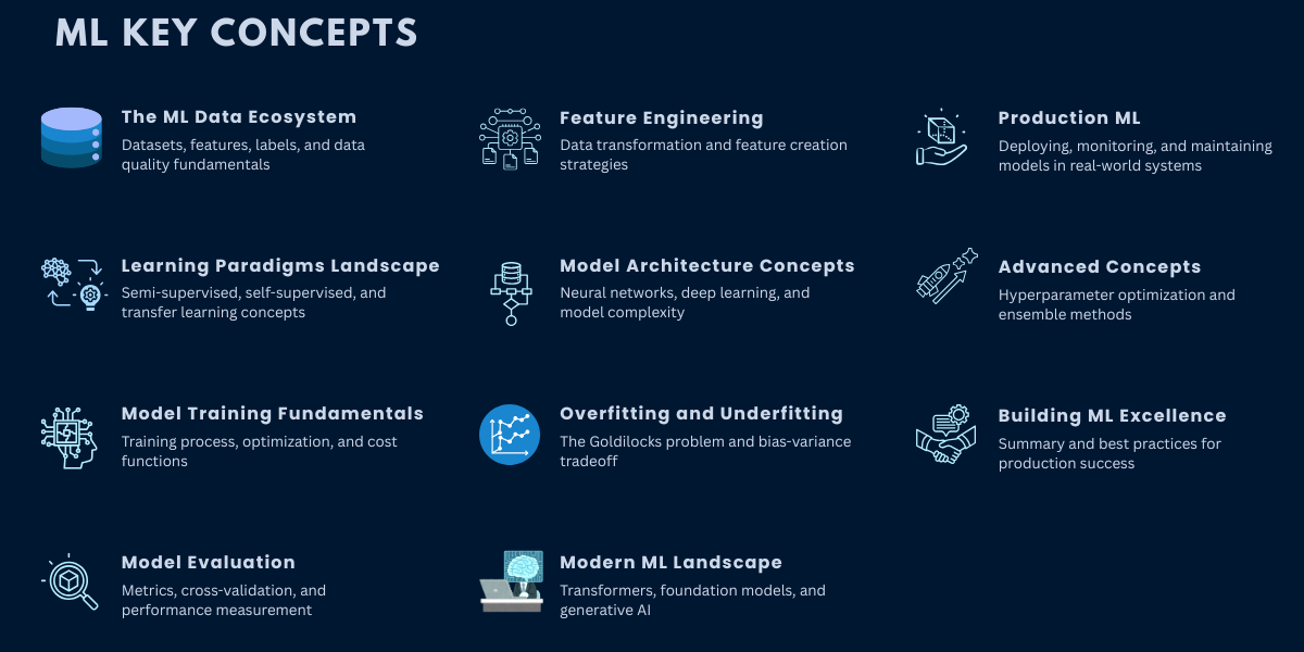
Essential ML Concepts Covered
01
Machine Learning Data Fundamentals - Understanding datasets, features, labels, and data quality essentials
02
Advanced Learning Paradigms - Semi-supervised, self-supervised, and transfer learning explained
03
Model Training and Optimization - How models learn through gradient descent, cost functions, and optimization
04
Model Evaluation Techniques - Metrics, cross-validation, and performance measurement methods
05
Feature Engineering and Selection - Transforming raw data into predictive features for better models
06
Neural Network Architectures - Deep learning vs classical ML, neural networks, and model complexity
07
Overfitting and Underfitting - Understanding bias-variance tradeoff and model generalization
08
Modern ML and Generative AI - Transformers, foundation models, prompt engineering, and GPT explained
09
Production ML Deployment - Scaling models, monitoring performance, and handling data drift
10
Advanced ML Techniques - Hyperparameter optimization and ensemble learning methods
11
ML Best Practices - Key takeaways and principles for production ML success
Machine Learning Data Fundamentals: Datasets, Features, and Labels Explained
Data is the fuel of machine learning, but not all data is created equal. Understanding how to categorize, evaluate, and prepare your data determines the ceiling of what your models can achieve.
Understanding Training, Validation, and Test Datasets in Machine Learning
A dataset is your collection of observations, but the devil is in the details. Netflix uses 130+ different datasets to power their recommendation engine, each carefully curated for specific ML tasks.
Dataset Type
Purpose
Industry Example
Key Characteristics
Training Set
Model Learning
Netflix's viewing history (80%)
Large, representative, clean
Validation Set
Hyperparameter Tuning
Spotify's skip prediction (10%)
Unseen during training, balanced
Test Set
Final Evaluation
Airbnb's price optimization (10%)
Completely hidden, real-world distribution
Holdout Set
Production Readiness
Uber's demand forecasting
Time-based split, business validation
Source: Analysis based on Netflix Technology Blog and Spotify Research publications (2019-2024)
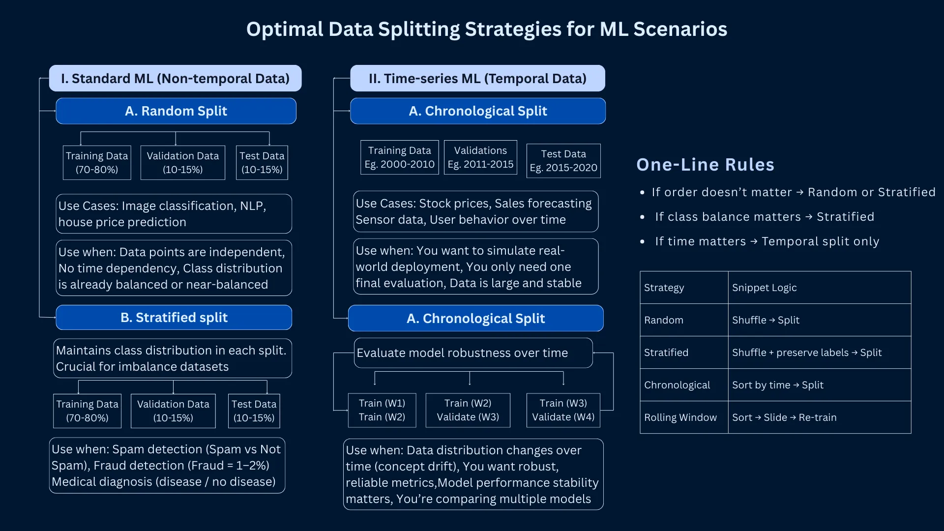
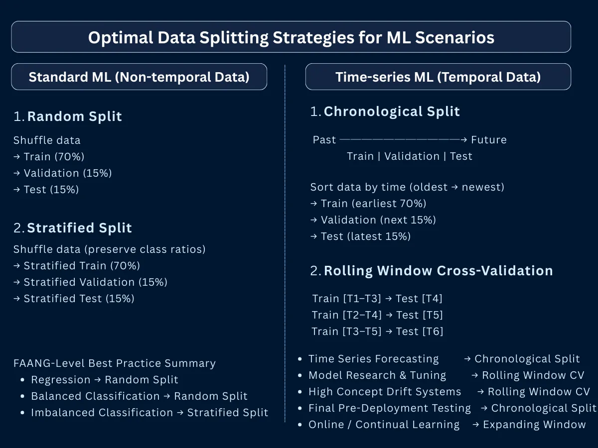
Optimal Data Splitting Strategies - Detailed breakdown showing train/validation/test splits for different ML scenarios with industry examples from FAANG companies
Data Splitting Strategies - Quick reference guide for choosing the right split ratio based on dataset size and problem complexity
What are Features in Machine Learning: Types and Applications
Features are the individual pieces of information that describe your data-think of them as the characteristics or attributes you measure. For example, when predicting house prices, features include square footage, number of bedrooms, location, and age of the house. Each feature is a single measurable property that helps the model understand and make predictions. Google's search ranking algorithm uses over 200 features to determine which websites to show you, while Tesla's Full Self-Driving system processes 8,000+ features per second from camera and sensor data.
Feature Type
Definition
Example
ML Applications
Numerical
Continuous or discrete numbers
Age, price, temperature
Linear regression, neural networks
Categorical
Discrete categories or classes
Color, brand, city
Decision trees, one-hot encoding
Ordinal
Categories with inherent order
Rating (1-5), size (S/M/L)
Ordinal encoding, tree-based models
Boolean
True/false binary values
Is_premium, has_discount
Logistic regression, SVMs
Text
Unstructured textual data
Reviews, descriptions, emails
NLP, embeddings, transformers
Image
Pixel arrays and visual data
Photos, medical scans, satellite imagery
CNNs, computer vision
Time Series
Temporal sequence data
Stock prices, sensor readings
RNNs, LSTMs, time series models
Source: Analysis based on Google AI, Tesla AI Day presentations, and industry ML practices (2020-2024)
Machine Learning Labels and Target Variables: Explicit vs Implicit Labeling
Labels (also called targets or outputs) are the correct answers you want your model to learn to predict. In supervised learning, each training example has both features (the input data) and a label (the correct answer). For instance, in an email spam detector, the label would be "spam" or "not spam" for each email. In a house price predictor, the label is the actual sale price. Labels are what teach your model what the right predictions should look like.
Production Insight: LinkedIn found that implicit labels (user engagement) often outperform explicit labels (user ratings) for recommendation systems, leading to significant improvements in click-through rates.
Advanced Machine Learning Paradigms: Semi-Supervised, Self-Supervised, and Transfer Learning
While supervised, unsupervised, and reinforcement learning form the foundation (covered in ML Fundamentals), modern ML systems increasingly rely on hybrid approaches that combine multiple learning paradigms for superior performance.
What is Semi-Supervised Learning: Combining Labeled and Unlabeled Data
Semi-supervised learning combines small amounts of labeled data with large amounts of unlabeled data. Google's "Noisy Student" approach achieved state-of-the-art ImageNet accuracy by training on 300M unlabeled images alongside standard labeled dataset.
Aspect
Supervised Learning
Semi-Supervised Learning
Key Advantage
Data Requirements
100% labeled data
10-30% labeled + unlabeled
90% reduction in labeling costs
Typical Use Case
Image classification
Medical image analysis
Expert labeling is expensive
Training Complexity
Straightforward
Moderate (pseudo-labeling)
Scales to larger datasets
Performance
High with enough labels
Approaches supervised with less labels
Cost-effective accuracy
Industry Example
Gmail spam detection
Google's content moderation
Handles scale economically
Source: Analysis based on Google AI Research and semi-supervised learning literature (2020-2024)
Production Strategy: Meta's content moderation system uses semi-supervised learning to handle 100+ languages, significantly reducing annotation costs while maintaining high accuracy across diverse linguistic contexts.
Self-Supervised Learning Explained: How GPT and BERT Learn Without Labels
Self-supervised learning creates its own labels from data structure. This paradigm powers modern LLMs like GPT-4 and BERT, which learn language patterns by predicting masked words or next tokens without human-labeled data.
The breakthrough: GPT-3 trained on 300B tokens with zero human labels, learning grammar, facts, and reasoning purely from predicting the next word. This approach scales to trillion-parameter models impossible to train with supervised learning.
Self-Supervised Task
How It Works
What Model Learns
Industry Application
Next Token Prediction
Predict next word in sequence
Language patterns, grammar, context
GPT-4, ChatGPT (OpenAI)
Masked Language Modeling
Predict randomly masked words
Bidirectional context, semantics
BERT, RoBERTa (Google, Meta)
Contrastive Learning
Similar images get similar embeddings
Visual representations, object features
CLIP, DALL-E (OpenAI)
Image Rotation Prediction
Predict rotation angle of image
Spatial relationships, object structure
SimCLR (Google Research)
Video Frame Prediction
Predict next frame in sequence
Motion patterns, temporal dynamics
Sora, autonomous driving (Tesla)
Source: Analysis based on OpenAI, Google Research, and Meta AI publications (2019-2024)
2024 Breakthrough: OpenAI's GPT-4 demonstrates that self-supervised learning at sufficient scale develops emergent abilities-capabilities like reasoning and mathematical problem-solving never explicitly trained, appearing only in models beyond 100B parameters.
Transfer Learning in Machine Learning: Fine-Tuning Pre-Trained Models
Transfer learning takes knowledge from one task and applies it to another. Instead of training from scratch, you start with a pre-trained model and fine-tune it for your specific needs-reducing training time from months to hours.
The economic impact is massive: Training GPT-3 from scratch costs $4-5M in compute. Fine-tuning it for your specific task costs $100-1,000. Transfer learning democratized AI by making powerful models accessible to organizations without massive compute budgets.
Transfer Learning Type
Scenario
Training Cost
Real Example
Feature Extraction
Use pre-trained layers as features
1-10% of from-scratch cost
Tesla's autopilot: ImageNet features for road detection
Fine-tuning
Adjust pre-trained model weights
5-20% of from-scratch cost
Hugging Face models: BERT fine-tuned for sentiment analysis
Domain Adaptation
Adapt model to new domain
10-30% of from-scratch cost
Medical imaging: Natural image models adapted to X-rays
Few-shot Learning
Learn from handful of examples
<1% of from-scratch cost
GPT-4: 5 examples in prompt teach new task
Zero-shot Learning
Perform task with no examples
No additional training
CLIP: Classify images it never saw during training
Source: Analysis based on OpenAI, Hugging Face, and transfer learning research (2020-2024)
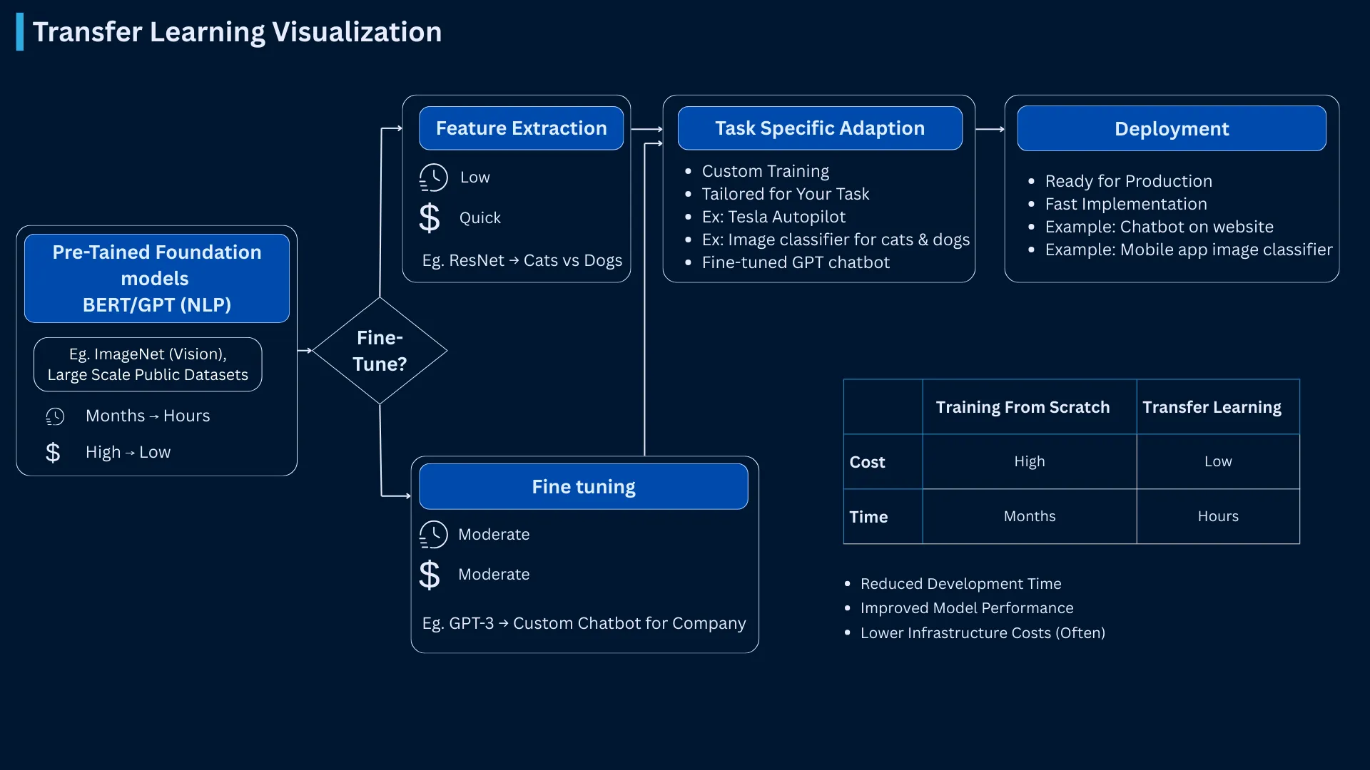
Transfer Learning Pipeline - Complete workflow from foundation models (ImageNet, GPT) through feature extraction and fine-tuning to deployment, with real-world cost and time comparisons
How Machine Learning Models Train: Optimization, Gradient Descent, and Cost Functions
Machine Learning Training Process: From Data to Predictions
Training is the learning phase where a machine learning algorithm studies your data and discovers patterns within it. During training, the algorithm repeatedly looks at examples, makes predictions, measures how wrong those predictions are, and then adjusts its internal settings to improve. This cycle continues thousands or millions of times until the model becomes good at making accurate predictions. For example, Google's BERT model required 4 days of continuous training on 64 specialized chips, processing 3.3 billion parameters to achieve human-level language understanding.
ML
ML Training Pipeline
Complete end-to-end machine learning workflow - click to expand details
1
Raw Data Ingestion
Collect and load data from various sources
2
Feature Engineering
Transform raw data into meaningful features
3
Model Training
Learn patterns from data via gradient descent
4
Validation
Evaluate performance on unseen data
5
Optimization Loop
Tune hyperparameters and iterate
6
Deployment
Deploy model to production systems
Production Reality: Companies like Google and Netflix run this pipeline continuously. BERT trained for 4 days on 64 TPUs (stages 2-4), while Netflix retrains recommendation models every few hours. Modern MLOps platforms like Kubeflow and SageMaker automate this entire workflow with monitoring at each stage.
6
Pipeline Stages
100s
Training Epochs
∞
Optimization Loop
Machine Learning Optimization: Adjusting Parameters to Minimize Error
Optimization is the core process that makes machine learning work. It's the method of systematically adjusting your model's internal parameters (weights and biases) to minimize the difference between predicted outputs and actual correct answers. Think of it like tuning a radio: you turn the dial slightly in different directions until you find the clearest signal. In machine learning, optimization algorithms automatically "turn the dials" of your model thousands or millions of times, each time getting closer to the best possible predictions.
Gradient Descent Algorithm: SGD, Mini-Batch, and Adam Optimizer Explained
Gradient descent is the workhorse optimization algorithm powering most ML models. Imagine you're blindfolded on a mountain, trying to reach the valley below. You feel the slope around you and take a step in the steepest downward direction. Repeat until you can't go lower-you've found the valley (optimal solution). Likewise, the gradient descent algorithm helps us find the lowest prediction error by iteratively moving toward better model parameters.
Gradient Descent Variant
How It Works
Key Trade-off
Used By
Batch Gradient Descent
Uses entire dataset per update
Accurate but slow, memory intensive
Small datasets, research experiments
Stochastic Gradient Descent (SGD)
Uses single example per update
Fast but noisy, requires tuning
Most production systems, proven reliability
Mini-batch Gradient Descent
Uses subset (32-512) per update
Balanced speed and stability
GPT-4, most deep learning (industry standard)
Adam Optimizer
Adaptive learning rates per parameter
Fast convergence, forgiving
Google's BERT, OpenAI's GPT series
AdaGrad
Adapts to sparse features
Good for NLP, can converge too fast
Google Ads, search ranking systems
Source: Analysis based on optimization algorithm research and production implementations (2017-2024)
Production Reality: Modern large language models like GPT-3 use adaptive optimizers like Adam for faster convergence compared to standard SGD. The right optimization algorithm significantly impacts training efficiency and compute costs at scale.
Machine Learning Loss Functions: MSE, Cross-Entropy, and Error Measurement
A cost function (also called a loss function or objective function) is the mathematical formula that measures how far your model's predictions are from the actual true values. Think of it as a scoring system that assigns a numerical penalty for every incorrect prediction-the larger the error, the higher the cost. The goal of training is to minimize this cost function, finding model parameters that produce the smallest possible error across all training examples.
Different problems require different cost functions because not all errors are equal. Predicting a house price $10,000 too high is a linear error, but misclassifying a cancerous tumor as benign could be fatal-requiring cost functions that heavily penalize false negatives. The choice of cost function fundamentally shapes what your model learns to optimize.
Cost Function
Problem Type
What It Measures
Industry Application
Mean Squared Error (MSE)
Regression
Average squared difference from true values
Uber's ETA prediction, stock price forecasting
Cross-Entropy Loss
Classification
Distance between probability distributions
Gmail spam detection, image classification
Binary Cross-Entropy
Binary Classification
Yes/no decision error
Netflix's click prediction, ad targeting
Hinge Loss
Support Vector Machines
Margin-based classification error
LinkedIn's job recommendation, text classification
Huber Loss
Robust Regression
Combines MSE and absolute error
Autonomous vehicles (handles sensor noise)
Source: Analysis based on cost function optimization research and ML systems design (2018-2024)
Learning Rate in Machine Learning: Balancing Training Speed and Convergence
Learning rate controls how big a step your model takes when adjusting its parameters during training. If the learning rate is too large, the model takes huge steps and might miss the best solution-like jumping over a target. If it's too small, the model takes tiny steps and training becomes extremely slow. Finding the right learning rate is essential for efficient training.
Convergence is the point when your model's training process stabilizes-when the cost function stops decreasing significantly and the model parameters stop changing substantially between training iterations. Think of it as reaching the destination: your model has found the best (or near-best) parameter values it can discover. A model that converges quickly is efficient, while a model that fails to converge wastes computational resources without improving performance.
Production Lesson: Learning rate scheduling (starting high, gradually reducing) has become standard practice in production systems for improved model convergence. Most modern deep learning systems use adaptive learning rate schedules rather than static values for better training stability and performance.
Common Machine Learning Algorithms: Decision Trees, Neural Networks, and Ensemble Methods
Algorithm Family
Learning Style
Best Use Cases
Industry Champions
Decision Trees
Rule-based splitting
Interpretable decisions, feature importance
Credit scoring (banks), medical diagnosis
Linear Models
Mathematical relationships
Baseline models, high-dimensional data
Google Ads bidding, financial modeling
Neural Networks
Complex pattern recognition
Image, text, speech processing
Facebook image tagging, Alexa speech
Ensemble Methods
Combined model power
Competitions, production systems
Netflix recommendations, Airbnb pricing
Support Vector Machines
Margin optimization
Text classification, bioinformatics
Gmail spam detection, drug discovery
Clustering Algorithms
Pattern discovery
Customer segmentation, anomaly detection
Spotify playlists, fraud detection
Source: Analysis based on company engineering blogs and ML conference proceedings (2018-2024)
Machine Learning Model Evaluation: Metrics, Cross-Validation, and Performance Measurement
Machine Learning Evaluation Metrics: Accuracy, Precision, Recall, and F1-Score
Choosing the right evaluation metric determines whether your model succeeds in production. Facebook's News Feed algorithm optimizes for time spent, while Netflix optimizes for completion rate-different metrics driving different behaviors.
Source: Analysis based on major tech companies' ML publications and fairness research (2019-2024)
Production Reality: Airbnb discovered that optimizing solely for booking rate led to lower host satisfaction. They now use multi-objective optimization balancing guest bookings with host preferences.
Cross-validation is a technique to get a more reliable estimate of how well your model will perform on new data. Instead of splitting your data just once into training and test sets, cross-validation splits it multiple times in different ways and tests the model on each split. This gives you a better sense of your model's true performance because you're testing it on multiple different subsets of data, not just one.
The most common approach is K-fold cross-validation: you divide your data into K equal parts (typically 5 or 10). The model trains on K-1 parts and tests on the remaining part. This repeats K times, with each part serving as the test set once. Finally, you average the K results to get an overall performance score. This method is more reliable than a single train-test split because it reduces the chance that your results are just lucky (or unlucky) based on how you happened to split the data.
Why This Visual? Choosing the wrong cross-validation strategy can lead to overoptimistic performance estimates and production failures. This interactive comparison helps you select the right approach based on your data characteristics, computational budget, and problem type. Click any strategy card below to see detailed pros/cons, use cases, and real company implementations.
Sort & Filter Strategies:
K-Fold Cross-Validation
+
Data is split into K equal-sized folds. The model is trained K times, each time using K-1 folds for training and 1 fold for validation.
Complexity:Medium
Variance Reduction:High
Stratified K-Fold
+
Enhanced K-Fold that preserves class distribution in each fold. Each fold maintains the same proportion of samples for each class as the complete dataset.
Complexity:Medium
Variance Reduction:Very High (for imbalanced data)
Time Series Split
+
Respects temporal ordering of data. Training set always precedes validation set in time. Multiple sequential train-test splits moving forward in time.
Complexity:Medium-High
Variance Reduction:Medium (realistic but high variance)
Group K-Fold
+
Ensures that samples from the same group appear only in one fold. Prevents data leakage when samples are related (e.g., multiple samples from same patient, user, or location).
Complexity:High
Variance Reduction:High (for grouped data)
Leave-One-Out CV (LOOCV)
+
Extreme case where K equals the number of samples. Each sample serves as the validation set exactly once while all others are used for training.
Complexity:Low (conceptually) / High (computationally)
Variance Reduction:Low (high variance estimate)
Nested Cross-Validation
+
Two-level CV: outer loop for performance estimation, inner loop for hyperparameter tuning. Prevents optimistic bias from hyperparameter search on the same data used for final evaluation.
Complexity:Very High
Variance Reduction:Very High (unbiased estimates)
Feature Engineering and Selection: Transforming Raw Data into Predictive Power
Feature Selection Methods: Filter, Wrapper, and Embedded Techniques
Feature selection is the process of choosing which features (input variables) are most useful for making accurate predictions. Not all features contribute equally-some might be highly predictive, while others add noise or redundancy. By selecting only the most important features, you can build simpler, faster models that often perform better because they focus on what truly matters.
Think of it like packing for a trip: you don't need to bring everything you own. Feature selection helps you identify the essentials. For example, when predicting house prices, square footage and location are critical features, but the color of the mailbox probably isn't. Spotify's recommendation engine uses sophisticated feature selection to choose from 10,000+ potential audio features, ultimately using only the ~100 most predictive ones-making their system both accurate and efficient.
Selection Method
Approach
Advantages
Use Cases
Filter Methods
Statistical tests (correlation, chi-square)
Fast, interpretable, model-agnostic
High-dimensional data, initial exploration
Wrapper Methods
Model performance-based selection
Optimal feature subsets, considers interactions
Small datasets, interpretable models
Embedded Methods
Built into model training (LASSO, Random Forest)
Automatic selection, efficient computation
Production systems, large-scale ML
Dimensionality Reduction
Transform to lower dimensions (PCA, t-SNE)
Removes noise, visualization, computation
Image processing, exploratory analysis
Source: Analysis based on Spotify ML research and feature engineering best practices (2020-2024)
Creating Engineered Features: Deriving New Variables for Better Predictions
Feature engineering is the creative process of creating new, more useful features from your existing raw data. Instead of just using the data as-is, you transform, combine, or derive new variables that make patterns easier for models to learn. This is often where the biggest performance improvements come from-more than just trying different algorithms.
For example, if you have a date field, you could engineer new features like "day of week," "is_weekend," "is_holiday," or "days_until_payday"-each capturing different patterns that might be predictive. Uber's demand forecasting creates 500+ engineered features from basic location and time data, including weather patterns, event calendars, and historical demand cycles. Good feature engineering turns simple data into rich, informative inputs that help models make better predictions.
Advanced Technique: Netflix engineers discovered that creating "viewing velocity" features (how quickly users consume content) significantly improved recommendation accuracy compared to basic viewing history alone.
Neural Network Architectures and Deep Learning vs Classical Machine Learning
Understanding model architecture helps you choose the right tool for your problem. The gap between classical ML and deep learning isn't just complexity-it's a fundamental shift in how models represent knowledge.
How Neural Networks Work: Layers, Neurons, and Hierarchical Learning
Neural networks are machine learning models inspired by how the human brain works. They consist of layers of interconnected "neurons" (simple processing units) that work together to learn patterns. Each neuron receives information, performs a simple calculation, and passes the result forward to neurons in the next layer. By connecting many of these simple neurons in layers, neural networks can learn to recognize complex patterns that would be impossible to program manually.
What makes neural networks powerful is their ability to learn in stages through multiple layers. For example, when recognizing faces in photos, the first layer might learn to detect simple edges and lines, the second layer combines these into shapes like eyes and noses, and the final layer recognizes complete faces. This step-by-step learning of increasingly complex features is what makes neural networks so effective for tasks like image recognition, speech understanding, and language translation.
Architecture Type
Structure
Best For
Industry Examples
Feedforward Networks
Simple input to hidden to output flow
Structured data, classification
Credit scoring, fraud detection
Convolutional Networks (CNNs)
Spatial pattern recognition layers
Images, visual data
Facebook's image tagging, medical imaging
Recurrent Networks (RNNs)
Sequential data with memory
Text, time series, speech
Google Translate, Siri speech recognition
Transformers
Parallel attention mechanisms
Language, multimodal tasks
ChatGPT, DALL-E, GPT-4
Graph Neural Networks
Relationship-based learning
Social networks, molecules
LinkedIn's connection recommendations
Source: Analysis based on neural network architecture research and applications (2012-2024)
Deep Learning vs Classical Machine Learning: When to Use Each Approach
Deep learning is a subset of machine learning that uses neural networks with many layers (hence "deep") to automatically learn complex patterns from large amounts of data. Classical machine learning refers to traditional algorithms like decision trees, linear regression, and support vector machines that typically require manual feature engineering and work well with smaller datasets.
The key difference: deep learning can automatically discover useful features from raw data (like learning to detect edges, shapes, and objects from pixels), while classical ML requires you to manually create those features. However, deep learning needs massive amounts of data and computational power to work well. Classical ML is often better for smaller datasets, faster training, and situations where you need to explain exactly how the model makes decisions. The choice depends on your data size, problem complexity, and business requirements.
Aspect
Classical ML
Deep Learning
Decision Factor
Data Requirements
100s to 100Ks of examples
Millions of examples needed
Small data favors classical ML
Feature Engineering
Manual feature creation critical
Automatic feature learning
Domain expertise vs data volume
Interpretability
Highly interpretable (trees, linear)
Black box (hard to explain)
Regulated industries need classical ML
Training Time
Minutes to hours
Hours to weeks
Production speed requirements
Hardware Needs
CPU sufficient
GPU/TPU essential
Infrastructure budget
Performance Ceiling
Good with modest data
Superior with massive data
Asymptotic performance needs
Source: Analysis based on ML systems comparison research and production trade-offs (2019-2024)
Production Decision: Airbnb uses classical ML (gradient boosted trees) for pricing because they have 150K listings (modest data) and need interpretability for host trust. Netflix uses deep learning for recommendations because they have 230M+ users generating billions of interactions-data volume justifies complexity.
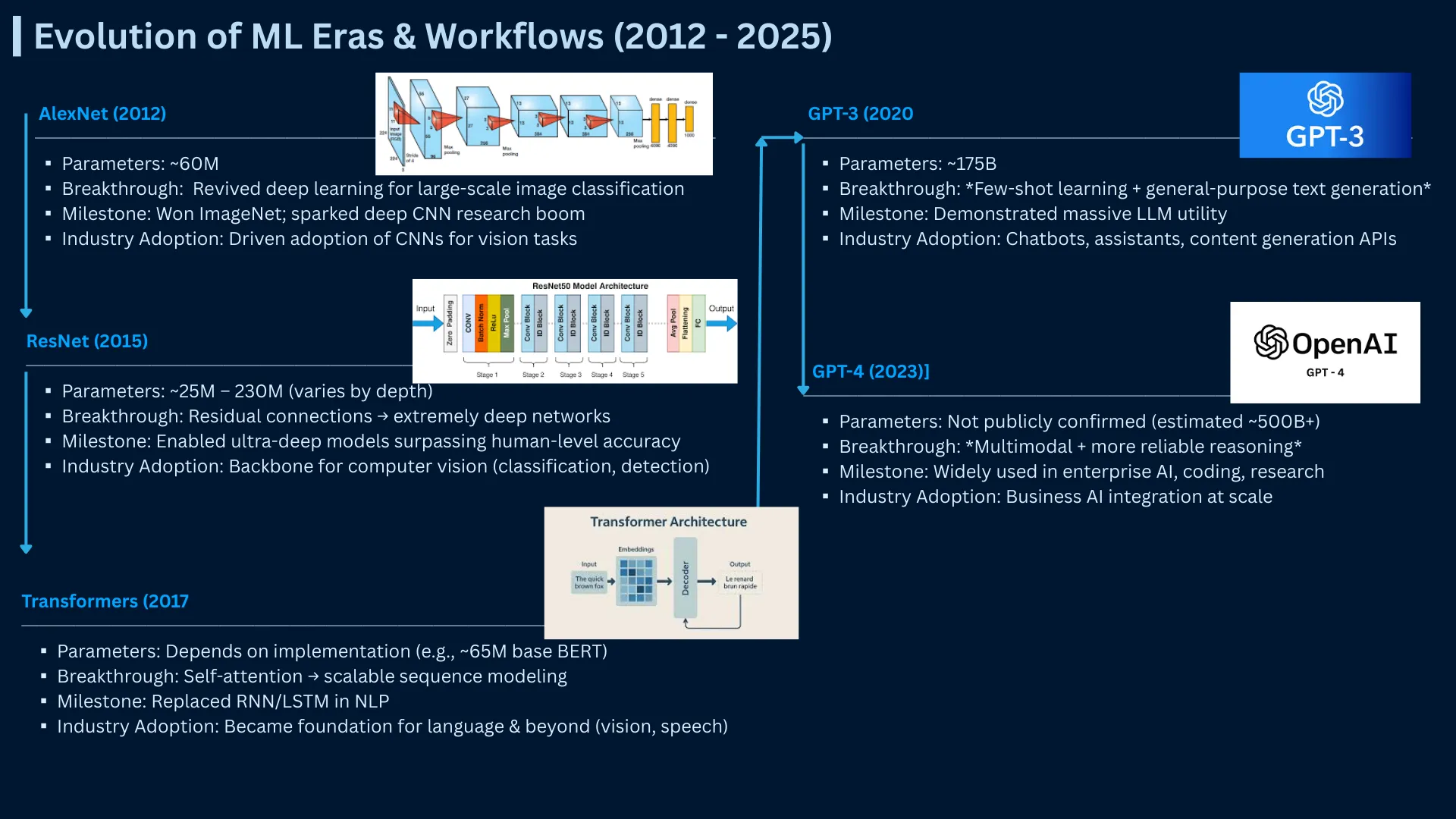
Model Complexity and Parameter Count: From Small to Frontier Models
Model capacity refers to the complexity a model can represent, primarily determined by parameter count. GPT-3's 175B parameters can capture nuanced language patterns, while a simple linear regression with 10 parameters handles basic relationships.
Model Scale
Parameter Range
Training Requirements
Use Cases
Tiny Models
1K - 1M parameters
CPU, minutes to hours
Mobile apps, edge devices, simple tasks
Small Models
1M - 100M parameters
Single GPU, hours to days
Most business ML, startups, MVPs
Medium Models
100M - 10B parameters
Multi-GPU, days to weeks
BERT, production NLP, computer vision
Large Models
10B - 100B parameters
GPU clusters, weeks
GPT-3, advanced AI applications
Frontier Models
100B+ parameters
Supercomputers, months
GPT-4, Claude, Gemini (research labs only)
Source: Analysis based on model scaling research and computational requirements (2020-2024)
ML Architecture Evolution (2012-2024) - From AlexNet to GPT-4 showing parameter growth, breakthrough capabilities, and industry adoption milestones across three eras
Overfitting and Underfitting: Finding the Right Model Complexity
Understanding Bias-Variance Tradeoff in Machine Learning Models
Overfitting happens when your model learns the training data too well-it memorizes specific examples including noise and random variations, rather than learning the general patterns. Imagine a student who memorizes exam answers word-for-word but doesn't understand the concepts-they'll fail when asked slightly different questions. An overfit model performs excellently on training data but poorly on new, unseen data.
Underfitting is the opposite problem: your model is too simple to capture the important patterns in your data. It's like trying to fit a straight line through data that clearly curves-you'll miss the relationship. An underfit model performs poorly on both training data and new data because it hasn't learned enough.
The goal is to find the sweet spot between these extremes-a model complex enough to learn the real patterns but simple enough not to memorize noise. This balance is one of machine learning's central challenges, often called the bias-variance tradeoff.
Problem
Symptoms
Solutions
Industry Example
Overfitting
High training accuracy, low test accuracy
Regularization, cross-validation, more data
Google's early PageRank: Reduced from 500 to 200 features
Underfitting
Low training and test accuracy
More features, complex models, better data
Netflix's initial collaborative filtering: Added content features
Source: Analysis based on Google Research publications and Netflix Technology Blog (2015-2024)
Explore the fundamental tradeoff: Use the slider below to adjust model complexity and watch how bias and variance change. Find the sweet spot where total error is minimized - this is the key to building models that generalize well to new data.
Bias (Underfitting Error)
Variance (Overfitting Error)
Total Error
Adjust Model Complexity
50%
SimpleComplex
Underfitting
Optimal
Overfitting
Bias Error
30.0%
Variance Error
24.1%
Total Error
54.1%
Optimal Zone
Best balance between bias and variance
Technical Example
Well-tuned ensemble with proper regularization
Industry Case Study
Google's PageRank: 200 carefully selected features
How to Address This:
Maintain this balance: You're in the sweet spot for generalization
Use cross-validation: Verify performance across multiple data splits
Monitor in production: Watch for data drift that might shift optimal complexity
A/B test carefully: Small changes could move you out of optimal zone
Transformers, Foundation Models, and Generative AI: The Modern Machine Learning Era
Machine learning has fundamentally transformed since 2017. The transformer revolution, foundation models, and generative AI have redefined what's possible-and what practitioners need to understand to stay relevant.
Transformer Architecture and Attention Mechanism: How GPT and BERT Work
Transformers are a type of neural network architecture that revolutionized how AI understands language. Unlike older approaches that read text one word at a time (like reading a book sequentially), transformers can look at all words in a sentence simultaneously and understand how they relate to each other. This makes them much faster and better at understanding context. Models like ChatGPT, GPT-4, and BERT are all built using transformer architecture.
The key innovation in transformers is the attention mechanism-it allows the model to focus on the most relevant words when understanding each part of a sentence. For example, in the sentence "The animal didn't cross the street because it was too tired," the attention mechanism helps the model understand that "it" refers to "the animal" and not "the street." This ability to understand relationships between words, even when they're far apart, is what makes transformers so powerful for language tasks.
Transformer Innovation
What It Enables
Breakthrough Model
Industry Impact
Self-Attention
Every word attends to every other word
BERT (2018)
Google Search understanding improved 10%
Parallel Processing
100x faster training than RNNs
GPT-2 (2019)
Made large-scale language models feasible
Scalability
Performance improves with more parameters
GPT-3 (2020)
Unlocked few-shot learning capabilities
Multimodal Attention
Connect text, images, audio
CLIP, DALL-E (2021)
Text-to-image generation became production-ready
Long Context
Process 100K+ tokens at once
Claude, GPT-4 (2023-24)
Analyze entire codebases or books
Source: Analysis based on transformer architecture research and evolution (2017-2024)
2024 State-of-the-Art: Claude 3.5 and GPT-4 Turbo process 200K tokens (150K words)-equivalent to a 500-page novel-in a single context window. This was impossible with pre-transformer architectures, which struggled beyond 1,000 words.
What are Foundation Models: Pre-Training and Fine-Tuning Large Language Models
Foundation models are large-scale models pre-trained on massive datasets, then adapted to countless downstream tasks. Rather than training from scratch for each use case, organizations fine-tune foundation models-democratizing access to state-of-the-art AI.
The economics are transformative: Training GPT-4 cost an estimated $100M. Fine-tuning it for your specific task costs $500-5,000. Foundation models make advanced AI accessible to companies without supercomputer budgets.
Foundation Model Type
Examples
Pre-training Data
Adaptation Methods
Language Models
GPT-4, Claude, Llama
Trillions of web text tokens
Prompt engineering, fine-tuning, RAG
Vision Models
CLIP, SAM (Segment Anything)
Billions of image-text pairs
Transfer learning, zero-shot classification
Multimodal Models
GPT-4V, Gemini, Claude 3
Text, images, code combined
Visual question answering, document analysis
Code Models
GitHub Copilot, CodeLlama
Billions of lines of code
Code completion, bug detection, translation
Embedding Models
OpenAI Ada, Cohere
Semantic relationship training
Search, recommendation, clustering
Source: Analysis based on foundation model research and commercial deployments (2021-2024)
Generative AI vs Discriminative Models: Understanding the Key Differences
Traditional ML is discriminative-it classifies, predicts, and recognizes patterns in existing data. Generative AI creates new content: text, images, code, music, video. This fundamental shift from "understanding" to "creating" unlocked entirely new application categories.
Aspect
Discriminative ML
Generative AI
Business Implication
Primary Function
Classify, predict, analyze
Create, synthesize, generate
Automation vs augmentation
Input-Output
Data to Label/Prediction
Prompt to Novel Content
Different value propositions
Training Data
1K-1M labeled examples
Billions of unlabeled examples
Data requirements differ vastly
Business Models
Efficiency, cost reduction
Creative work, content creation
Revenue vs cost savings focus
Examples
Spam detection, fraud detection
ChatGPT, DALL-E, GitHub Copilot
Different competitive moats
Market Size
$150B ML market (2024)
$1.3T generative AI by 2032
Generative AI growing 10x faster
Source: Analysis based on Bloomberg Intelligence, McKinsey, and AI market research (2023-2024)
Production Reality: Shopify uses discriminative ML for fraud detection (reduces losses) and generative AI for product descriptions (increases revenue). Both are critical, but generative AI opened new revenue streams rather than just optimizing costs.
Prompt Engineering Techniques: Zero-Shot, Few-Shot, and Chain-of-Thought
Prompt engineering is the skill of writing effective instructions for AI models like ChatGPT or GPT-4. Instead of training a new model from scratch (which requires thousands of labeled examples and computational resources), you simply write clear, well-structured prompts that guide the AI to produce the results you want. A good prompt can make the difference between getting useless output and getting exactly what you need.
For example, instead of saying "write about dogs," a better prompt would be "write a 3-paragraph explanation of why dogs make good family pets, focusing on their loyalty, trainability, and companionship." The more specific and clear your instructions, the better the AI's response. This approach is faster and cheaper than traditional machine learning for many tasks.
Technique
What It Does
Use Case
vs Traditional ML
Zero-shot Prompting
Task with no examples
Quick prototypes, general tasks
0 labeled examples vs 1,000+
Few-shot Prompting
Task with 3-10 examples
Domain-specific classification
10 examples vs 10,000+
Chain-of-Thought
Break reasoning into steps
Math, logic, complex reasoning
Emergent capability, no training
RAG (Retrieval)
Inject relevant context
Document QA, knowledge bases
No retraining needed for updates
Fine-tuning
Adapt model with 100s of examples
Specialized tone, format, domain
10-100x cheaper than training
Source: Analysis based on prompt engineering research and LLM optimization techniques (2022-2024)
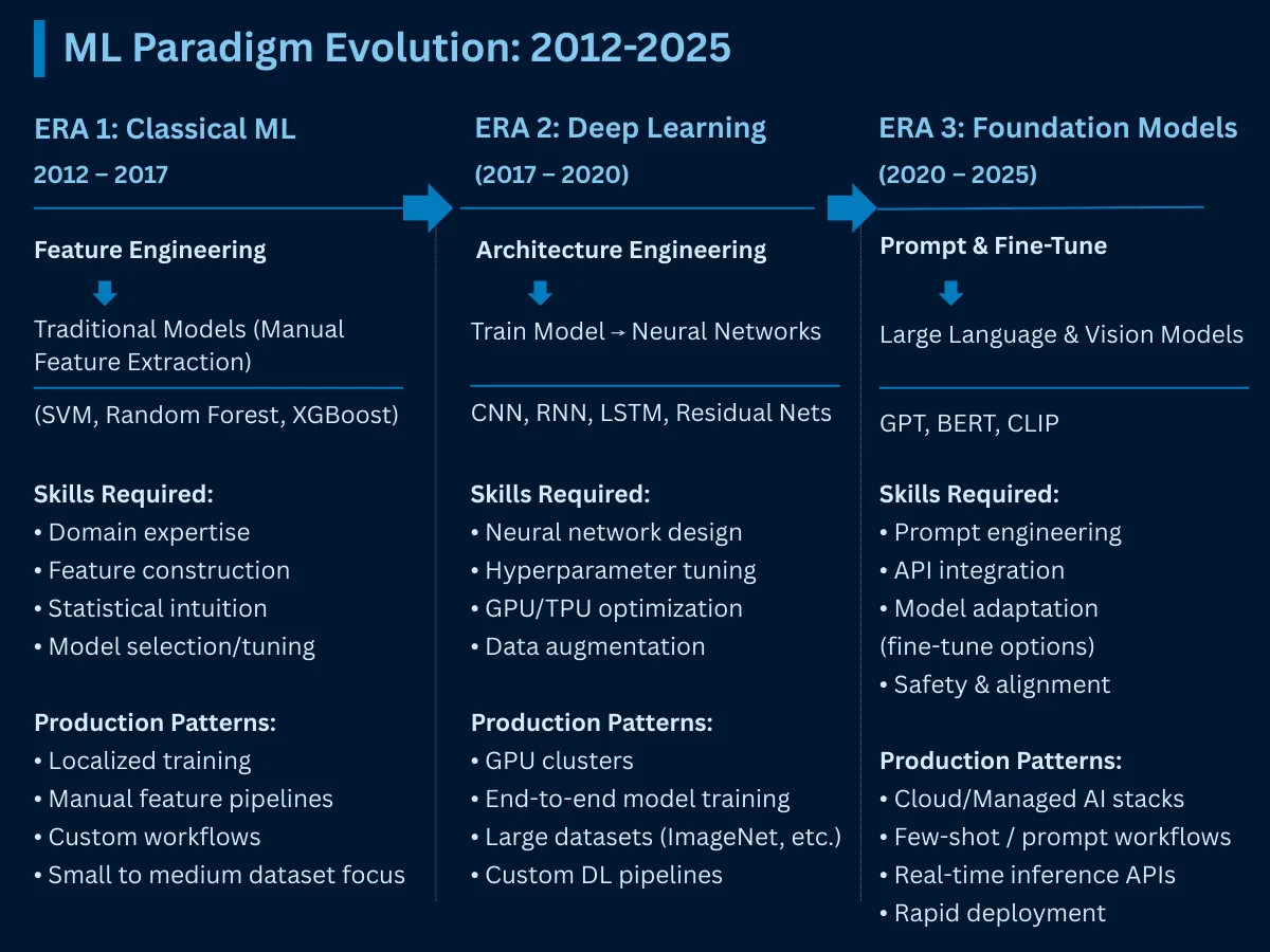
ML Paradigm Evolution (2012-2025) - Three transformative eras showing the shift from feature engineering to architecture engineering to prompt engineering, with production pattern changes
Deploying Machine Learning Models in Production: Scaling, Monitoring, and Data Drift
ML Model Deployment Strategies: Latency, Throughput, and Scalability
Model deployment is the process of taking your trained machine learning model and putting it into a real application where actual users can interact with it. This is different from training and testing in a controlled environment. When deployed, your model needs to respond quickly (often in milliseconds), handle many users at once, and work reliably 24/7. Deployment involves setting up servers, monitoring performance, and ensuring the model continues to work well as real users send it new data.
Deployment Aspect
Key Considerations
Industry Standards
Example Implementation
Latency
Response time requirements
< 100ms (search), < 10ms (ads)
Google Search: 25ms average response
Throughput
Requests per second capacity
10K-1M+ QPS depending on application
Netflix: 15M+ recommendations/second
Model Freshness
How often models update
Hourly (ads) to monthly (recommendations)
Uber: Real-time pricing model updates
Monitoring
Performance tracking and alerts
99.9%+ uptime, drift detection
LinkedIn: Feature drift monitoring
Scalability
Handle traffic spikes and growth
Auto-scaling, load balancing
Amazon: Prime Day traffic 10x scaling
Source: Analysis based on major tech companies' infrastructure publications (2020-2024)
Data Drift Detection and Model Degradation in Production Systems
Data drift happens when the real-world data your model sees in production starts to look different from the data it was trained on. This causes your model's accuracy to gradually decrease over time. Think of it like learning to recognize cars from 1990s photos, then being asked to identify modern electric vehicles-the patterns have changed, so your knowledge becomes outdated.
For example, during COVID-19, Uber's ride demand prediction models stopped working well because people's travel patterns completely changed overnight. What used to predict rush hour demand accurately was now useless. Data drift is common in real applications because the world keeps changing-customer preferences shift, seasonal patterns change, and unexpected events happen. Good production systems monitor for drift and retrain models when needed.
Industry Lesson: Airbnb's pricing models experienced 40% accuracy drop during COVID-19 due to unprecedented booking pattern changes. They implemented automated drift detection triggering model retraining within 24 hours of significant changes.
Hyperparameter Optimization and Ensemble Methods for Advanced ML Performance
Hyperparameter Tuning Methods: Grid Search, Random Search, and Bayesian Optimization
Hyperparameters are the settings you configure before training your model-they control how the learning process works. Think of them like the settings on a camera: shutter speed, aperture, and ISO must be set before you take a photo. Similarly, hyperparameters like learning rate, number of layers, and batch size must be chosen before training begins. Unlike regular parameters (which the model learns during training), hyperparameters are chosen by you.
For example, the learning rate (how big each training step is) and number of epochs (how many times to go through the data) are hyperparameters. Choosing good hyperparameters can mean the difference between a model that takes days to train poorly and one that trains in hours with excellent results. Finding the best hyperparameters often requires experimentation-trying different combinations and seeing which works best, a process called hyperparameter tuning or optimization.
Why This Visual? This comparison matrix reveals cost-performance trade-offs across optimization techniques that text alone cannot convey clearly - helping you choose between grid search, random search, Bayesian optimization, and neural architecture search based on your specific constraints.
⚙
Quick Selection Guide
Small Dataset
Grid Search
Exhaustive is feasible
Limited Budget
Bayesian Opt
Smart sampling
Large Space
Random Search
Good coverage
SOTA Needed
NAS
Google-scale only
Grid Search
TRADITIONAL
▲
Cost: Very High
Accuracy: 100% (finds optimal within grid)
Scalability: Poor (exponential growth)
How It Works
Exhaustive search through manually specified hyperparameter combinations. Tests every possible combination in the search space.
Search Space: Discrete grid of predefined values
Performance Profile
Time Complexity
O(n^d) - exponential with dimensions
Dataset Size
Small to Medium (< 100K samples)
Compute Budget
High (hours to days acceptable)
Expertise Needed
Low (easy to understand and implement)
Best For
Small hyperparameter spaces (2-3 parameters)
Final tuning after initial exploration
Reproducible research experiments
When computational budget is unlimited
Limitations
Computationally expensive for large spaces
Misses optimal points between grid values
Inefficient - tests many poor combinations
Exponential cost with parameter count
Real-World Example
Sklearn's GridSearchCV with 3-fold CV on Random Forest (n_estimators=[100,200,300], max_depth=[10,20,30]) requires 27 model trainings. Used by data science teams for final model tuning.
Random Search
TRADITIONAL
▼
Cost: Medium to High
Accuracy: 85-95% (probabilistic coverage)
Scalability: Good (controllable iterations)
Bayesian Optimization
ADVANCED
▼
Cost: Medium
Accuracy: 90-98% (smart exploration)
Scalability: Excellent (efficient sampling)
Neural Architecture Search (NAS)
AUTOMATED
▼
Cost: Extremely High
Accuracy: 95-100% (can exceed human designs)
Scalability: Poor (requires massive compute)
Quick Comparison Matrix
Technique
Cost
Speed
Accuracy
Best Use Case
Grid Search
Very High
O(n^d)
100% (finds optimal within grid)
Small hyperparameter spaces (2-3 parameters)
Random Search
Medium to High
O(n)
85-95% (probabilistic coverage)
Large hyperparameter spaces (5+ parameters)
Bayesian Optimization
Medium
O(n^3) per iteration
90-98% (smart exploration)
Expensive model training (hours per trial)
Neural Architecture Search (NAS)
Extremely High
O(n * m)
95-100% (can exceed human designs)
Novel problem domains with unique requirements
Ensemble Learning Techniques: Bagging, Boosting, and Stacking Explained
Ensemble methods combine predictions from multiple models to make better decisions than any single model could achieve alone. Think of it like consulting multiple doctors before making a medical decision-each doctor might notice different symptoms or have different expertise, and together they provide a more accurate diagnosis than any one doctor alone.
For example, Random Forest (a bagging ensemble) trains hundreds of decision trees on different subsets of data, then averages their predictions. XGBoost (a boosting ensemble) trains trees sequentially, where each new tree focuses on correcting the mistakes of previous trees. These ensemble approaches are so effective that they dominate machine learning competitions and power systems like Netflix's recommendation engine, which combines 130+ specialized algorithms.
Ensemble Type
How It Works
Advantages
Industry Applications
Bagging
Train models on data subsets
Reduces overfitting, parallel training
Random Forest for credit scoring
Boosting
Sequential model improvement
High accuracy, handles bias
XGBoost for Kaggle competitions
Stacking
Meta-model combines base models
Leverages model diversity
Netflix recommendation blending
Voting
Democratic decision making
Simple, interpretable
Medical diagnosis systems
Mixture of Experts
Models specialize in data regions
Scales to large problems
Google Translate language routing
Source: Analysis based on ensemble learning research and production implementations (2018-2024)
Why This Visual? This interactive concept map reveals the dependencies and relationships between core ML concepts - showing how data preparation flows into feature engineering, which enables training, which requires evaluation before deployment in a way that static text cannot clearly convey.
ML Workflow Overview
Data Pipeline
Foundation
Preparation + Features
Model Development
Core Process
Training + Tuning
Evaluation
Validation
Metrics + Testing
Production
Deployment
Serving + Monitoring
Data Preparation
Data Pipeline
▲
The foundation of all ML projects - collecting, cleaning, and transforming raw data into a format suitable for model training.
Enables: Feature Engineering, Model Training
Key Principles
Quality over quantity - clean data beats big data
Representative sampling - data must reflect real-world distribution
Feature scaling - normalize numerical features for consistent learning
Train/validation/test splits - prevent data leakage
Common Challenges
Missing values and outliers requiring imputation strategies
Imbalanced datasets skewing model predictions
Data drift over time affecting model performance
Privacy and compliance constraints on data usage
Best Practices
Document all preprocessing steps for reproducibility
Netflix processes 1TB+ daily viewing data through automated pipelines that handle missing timestamps, filter bot traffic, and normalize user engagement metrics before feeding into recommendation models.
Feature Engineering
Data Pipeline
▼
Creating informative input variables from raw data - the art of transforming domain knowledge into mathematical representations that models can learn from.
Depends on: Data Preparation
Enables: Model Training, Model Evaluation
Model Training
Model Development
▼
The process of teaching algorithms to recognize patterns in data by iteratively adjusting parameters to minimize prediction errors.
Depends on: Data Preparation, Feature Engineering
Enables: Hyperparameter Tuning, Model Evaluation
Hyperparameter Tuning
Model Development
▼
Optimizing model configuration settings that control the learning process - finding the sweet spot between model complexity and generalization.
Depends on: Model Training
Enables: Model Evaluation
Model Evaluation
Evaluation & Validation
▼
Assessing model performance using appropriate metrics and validation strategies to ensure reliability before deployment.
Depends on: Feature Engineering, Model Training, Hyperparameter Tuning
Enables: Model Deployment
Model Deployment
Production Deployment
▼
Taking trained models from development to production - serving predictions reliably at scale with monitoring and governance.
Depends on: Model Evaluation
Complete ML Workflow
1
Data Preparation
Clean, transform, split data
→
2
Feature Engineering
Create informative features
→
3
Model Training
Learn patterns from data
→
4
Hyperparameter Tuning
Optimize configuration
→
5
Model Evaluation
Validate performance
→
6
Deployment
Serve predictions at scale
Machine Learning Best Practices: Key Takeaways for Production Success
Mastering these key ML concepts separates amateur experiments from professional production systems. Companies like Netflix, Google, and Uber succeed because they excel at the fundamentals: quality data preparation, appropriate algorithm selection, robust evaluation, and production-ready deployment.
Research Sources & Industry References
1.
"Netflix Technology Blog: Recommendation System Architecture and Feature Engineering"
Technical deep-dive into Netflix's recommendation system architecture, feature engineering practices, and A/B testing frameworks
2.
"Google AI Research: Machine Learning Systems Design and Production Best Practices"
Comprehensive guide to ML systems design, production deployment, and scalability considerations at Google scale
3.
"OpenAI Research: GPT Series, Self-Supervised Learning, and Foundation Models"
GPT architecture evolution, self-supervised learning techniques, scaling laws, and foundation model capabilities
4.
"Attention Is All You Need: Transformer Architecture"
Seminal paper introducing transformer architecture and attention mechanisms that revolutionized NLP and AI
5.
"Meta AI Research: Semi-Supervised Learning and Content Moderation Systems"
Semi-supervised learning applications, content moderation at scale, and multimodal model development
6.
"Uber Engineering: Real-time Machine Learning and Data Drift Detection"
Real-time ML pipeline architecture, data drift detection systems, and model monitoring frameworks
7.
"Spotify Research: Audio Feature Engineering and Recommendation Systems"
Audio feature selection techniques, recommendation algorithm optimization, and user behavior modeling
8.
"Hugging Face: Transfer Learning and Fine-tuning Methodologies"
Transfer learning best practices, fine-tuning techniques, and democratization of foundation models
9.
"Airbnb Data Science: Multi-objective Optimization and Model Evaluation"
Multi-objective optimization strategies, model evaluation frameworks, and business metrics integration
10.
"Tesla AI: Optimization Algorithms and Neural Network Training"
Learning rate scheduling, optimization strategies for autonomous driving, and production neural network architectures
11.
"LinkedIn Engineering: Feature Selection and Production ML Monitoring"
Large-scale feature selection methods, production ML monitoring, and performance optimization techniques
12.
"Amazon Science: Large-scale Recommendation Systems and Ensemble Methods"
Large-scale recommendation system design, ensemble learning methods, and personalization algorithms
13.
"CLIP and DALL-E: Contrastive Learning and Multimodal AI"
Contrastive learning for vision-language models and breakthrough text-to-image generation capabilities
14.
"Bloomberg Intelligence & McKinsey: Generative AI Market Analysis"
Economic impact analysis of generative AI, market size projections, and industry transformation insights
15.
"Prompt Engineering and Chain-of-Thought Reasoning Research"
Prompt engineering techniques, chain-of-thought reasoning, and LLM optimization strategies