Clustering Methods

Discover hidden groups and patterns in unlabeled data using proven clustering algorithms

Read 15 min

Unsupervised Learning K-Means Hierarchical Clustering DBSCAN Clustering

You've mastered supervised learning, where algorithms learn from labeled examples. Now explore the opposite: unsupervised learning, where algorithms discover patterns without any labels. Clustering is the most fundamental unsupervised learning task - finding natural groups in data when you don't know the groups in advance. When Netflix groups similar viewers, when Amazon segments customers by shopping behavior, when researchers discover new cancer subtypes from genetic data - that's clustering revealing hidden structure in unlabeled data.

What Makes This Tutorial Different

This page introduces the most important clustering algorithms for discovering groups in unlabeled data. You'll learn what clustering is, how it differs from classification, and when to use each major clustering method. We focus on high-level understanding and practical application, with detailed algorithm mechanics saved for dedicated deep-dive pages.

Abbreviations Used in This Article (11 abbreviations)

DBSCAN Density-Based Spatial Clustering of Applications with Noise

GMM Gaussian Mixture Models

EM Expectation-Maximization

PAM Partitioning Around Medoids

KNN K-Nearest Neighbors

SVM Support Vector Machine

PCA Principal Component Analysis

t-SNE t-Distributed Stochastic Neighbor Embedding

UMAP Uniform Manifold Approximation and Projection

LDA Linear Discriminant Analysis

OPTICS Ordering Points To Identify the Clustering Structure

What You'll Master in This Guide

What Is Clustering? - Understanding unsupervised grouping and pattern discovery

Clustering vs Classification - Key differences between supervised and unsupervised grouping

Common Clustering Algorithms - K-means, hierarchical, DBSCAN, and Gaussian mixture models

Choosing the Right Algorithm - Matching clustering methods to problem characteristics

Evaluating Clustering Quality - Metrics and techniques for assessing cluster validity

Real-World Applications - Where clustering excels in industry and research

Frequently Asked Questions - Common questions about clustering methods

Clustering is fundamental because it's how we make sense of the world. Every concept you have - from 'chair' to 'democracy' - is really a cluster of similar instances. When machines can cluster as well as humans do, they'll truly understand. The challenge isn't just finding clusters, it's finding the right clusters at the right level of abstraction.

Peter Norvig

Director of Research at Google, Co-author of AI: A Modern Approach

What Is Clustering?

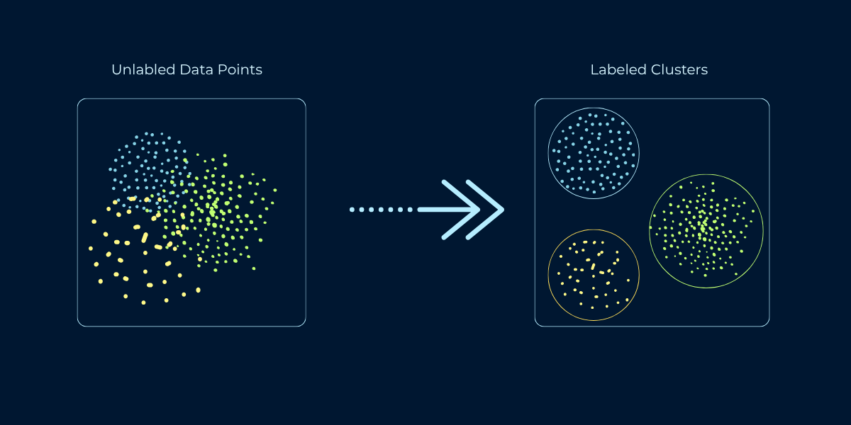
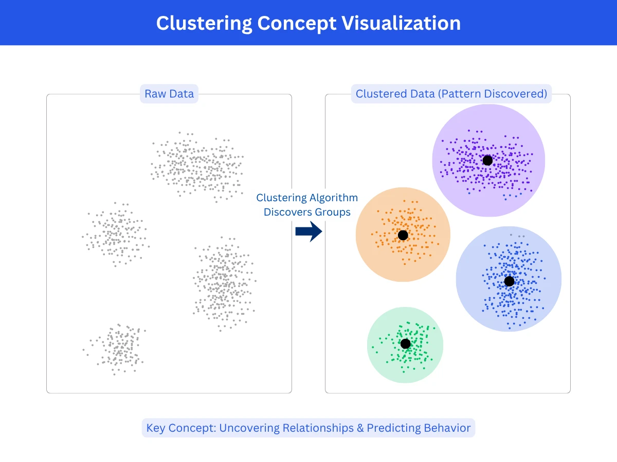
Clustering is the task of grouping similar data points together without predefined categories or labels. The algorithm examines features of your data and discovers natural groupings based on similarity. Points within a cluster should be similar to each other and different from points in other clusters. Unlike classification, where you predict which predefined category a data point belongs to, clustering discovers the categories themselves from the data's structure.

Think of organizing a photo library. Classification would be: given labeled categories (family, vacation, work), assign each new photo to a category. Clustering would be: look at all photos and group similar ones together, discovering natural categories like "beach photos," "indoor group shots," "sunset landscapes" without being told these categories exist. The algorithm finds structure you didn't know was there.

Side-by-side comparison of raw unlabeled data versus clustered data: left panel shows gray scatter plot points with no grouping, right panel shows same points color-coded into 3-4 distinct clusters with centroids marked and boundaries drawn — Clustering Concept Visualization - A clustering algorithm transforms unlabeled data (left) into meaningful groups with distinct boundaries (right)

Types of Clustering Problems

Partitional clustering: Divide data into non-overlapping groups where each point belongs to exactly one cluster. Example: k-means assigns every customer to one segment (budget, mid-tier, premium).
Hierarchical clustering: Build a tree of nested clusters, allowing different granularities. Example: biology taxonomy (species - genus - family - order) where clusters nest within larger clusters.
Density-based clustering: Find regions of high density separated by low-density regions. Points in sparse areas become outliers. Example: detecting fraud patterns - normal transactions cluster densely, fraudulent ones are sparse outliers.
Model-based clustering: Assumes each cluster has a natural shape and finds groups by fitting those shapes to the data. Example: if you plot customer spending, you might see two humps - frequent small purchases and occasional large ones. The algorithm fits a curve to each hump to define the groups, so a customer near the overlap can softly belong to both rather than being forced into one.

Clustering vs Classification: Key Differences

Clustering and classification both group data, but they approach the problem from opposite directions. Understanding this distinction is crucial for choosing the right technique for your problem.

Clustering vs Classification Comparison
Aspect	Classification (Supervised)	Clustering (Unsupervised)
Learning Type	Supervised - requires labeled training data	Unsupervised - no labels needed
Categories	Predefined - you specify categories in advance	Discovered - algorithm finds categories from data
Goal	Predict which known category new data belongs to	Discover unknown groups and patterns in data
Training Data	Examples with known labels (spam/not spam)	Just features, no labels
Number of Groups	Fixed - determined by training labels	Variable - you choose or algorithm decides
Evaluation	Accuracy against known labels	Cluster quality metrics (cohesion, separation)
Example	Classify email as spam using labeled training emails	Group customers by behavior without predefined segments

Source: Framework based on supervised vs unsupervised learning taxonomy

Quick Decision Rule

Ask: "Do I know the groups in advance?" If YES and you have labeled examples of each group, use classification. If NO and you want to discover natural groups from data, use clustering. If you have groups but no labels, try clustering first to discover structure, then potentially label clusters and switch to classification.

Common Clustering Algorithms

Different clustering algorithms make different assumptions about data structure. Understanding each algorithm's approach helps you choose the right one for your specific data characteristics and goals.

1. K-Means Clustering

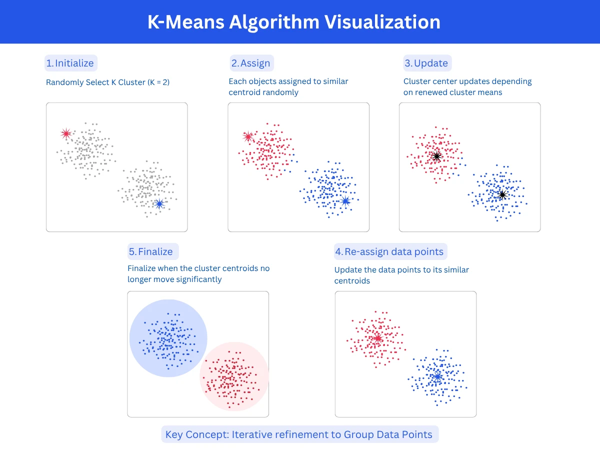
K-means is the most popular clustering algorithm due to its simplicity and speed. You specify K (the number of clusters), and the algorithm assigns each point to the nearest cluster center (Centroid), then iteratively refines centroids until Convergence. It works by minimizing the distance from points to their assigned centroid. The algorithm is fast, scales well to large datasets, and produces Spherical Clusters, evenly-sized clusters.

How it works: Initialize K random centroids, assign each point to nearest centroid, recalculate centroids as cluster means, repeat until centroids stabilize
Strengths: Very fast (scales to millions of points), simple to understand and implement, guaranteed to converge, works well for spherical clusters
Limitations: Must specify K in advance, assumes spherical equal-sized clusters, sensitive to initial centroid placement, struggles with irregular shapes
Best for: Large datasets, spherical well-separated clusters, when K is known or can be estimated
Common uses: Customer segmentation, image compression, document clustering, feature engineering

4-panel progression of the K-means algorithm: panel 1 shows random centroid initialization, panel 2 shows point assignment by nearest centroid, panel 3 shows centroid repositioning, panel 4 shows final converged clusters with stable boundaries — K-Means Algorithm Step-by-Step - The iterative process of Initialize, Assign, Update, and Converge until clusters stabilize

K-Means Clustering Implementation Python


            1
            from sklearn.cluster import KMeans
          

            2
            from sklearn.datasets import make_blobs
          

            3
            import matplotlib.pyplot as plt
          

            4
            import numpy as np
          

            5
            
          

            6
            # Generate synthetic data with 3 natural clusters
          

            7
            X, y_true = make_blobs(n_samples=300, centers=3, cluster_std=0.6, random_state=42)
          

            8
            
          

            9
            # Apply K-Means clustering
          

            10
            kmeans = KMeans(n_clusters=3, random_state=42, n_init=10)
          

            11
            kmeans.fit(X)
          

            12
            
          

            13
            # Get cluster assignments and centroids
          

            14
            labels = kmeans.labels_
          

            15
            centroids = kmeans.cluster_centers_
          

            16
            
          

            17
            print(f"Cluster assignments (first 10 points): {labels[:10]}")
          

            18
            # Output: [0 0 2 2 0 0 1 1 2 2]
          

            19
            
          

            20
            print(f"\nCluster centroids:")
          

            21
            for i, centroid in enumerate(centroids):
          

            22
                print(f"  Cluster {i}: [{centroid[0]:.2f}, {centroid[1]:.2f}]")
          

            23
            # Output:
          

            24
            #   Cluster 0: [-8.94, -8.48]
          

            25
            #   Cluster 1: [4.02, -8.08]
          

            26
            #   Cluster 2: [1.83, -0.15]
          

            27
            
          

            28
            # Evaluate clustering quality
          

            29
            inertia = kmeans.inertia_  # Sum of squared distances to nearest centroid
          

            30
            print(f"\nInertia (lower is better): {inertia:.2f}")  # Output: 327.45
          

            31
            
          

            32
            # Predict cluster for new point
          

            33
            new_point = [[0, 0]]
          

            34
            predicted_cluster = kmeans.predict(new_point)
          

            35
            print(f"\nNew point [0, 0] belongs to cluster: {predicted_cluster[0]}")

This example clusters 300 points into 3 groups using K-Means. The algorithm converges quickly (typically 5-10 iterations) and assigns each point to the nearest centroid. Inertia measures cluster compactness - lower values indicate tighter clusters. K-Means works best when clusters are spherical and roughly equal-sized, as shown here.

2. Hierarchical Clustering

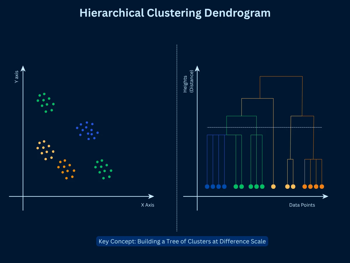
Hierarchical clustering builds a tree (Dendrogram) of nested clusters, allowing you to view data at multiple Granularity. Two approaches exist: Agglomerative (bottom-up: start with each point as a cluster, merge similar clusters) and divisive (top-down: start with one cluster, split recursively). Agglomerative is more common. The dendrogram shows the merge sequence, and you can cut at any height to get different numbers of clusters.

How it works: Start with N clusters (one per point), merge the two most similar clusters, repeat until one cluster remains, cut dendrogram at desired height
Strengths: Don't need to specify K upfront, produces hierarchical structure showing relationships, deterministic results, works with any distance metric
Limitations: Slow on large datasets (O(n^3) complexity), merge decisions are final (can't undo bad early merges), memory intensive
Best for: Small to medium datasets, when cluster hierarchy matters, exploratory analysis to determine K, taxonomies
Common uses: Gene expression analysis, species classification, document organization, social network analysis

Hierarchical clustering dendrogram showing scatter plot data points on the left and tree diagram on the right, with individual points as leaves merging upward into clusters, a horizontal cut line showing 3 final clusters, and branches color-coded by cluster assignment — Hierarchical Clustering Dendrogram - The tree structure reveals cluster relationships at every level, letting you choose how many groups to extract with a single cut

Hierarchical Clustering with Dendrogram Analysis Python


            1
            from sklearn.cluster import AgglomerativeClustering
          

            2
            from scipy.cluster.hierarchy import dendrogram, linkage
          

            3
            import numpy as np
          

            4
            
          

            5
            # Generate sample data
          

            6
            X = np.array([[0, 0], [0, 1], [1, 0],
          

            7
                          [5, 5], [5, 6], [6, 5],
          

            8
                          [10, 10], [10, 11], [11, 10]])
          

            9
            
          

            10
            # Perform hierarchical clustering (agglomerative)
          

            11
            hierarchical = AgglomerativeClustering(n_clusters=3, linkage='ward')
          

            12
            labels = hierarchical.fit_predict(X)
          

            13
            
          

            14
            print(f"Cluster assignments: {labels}")
          

            15
            # Output: [0 0 0 1 1 1 2 2 2]
          

            16
            
          

            17
            # Create linkage matrix for dendrogram visualization
          

            18
            linkage_matrix = linkage(X, method='ward')
          

            19
            
          

            20
            print(f"\nLinkage matrix (last 5 merges):")
          

            21
            print(linkage_matrix[-5:])
          

            22
            # Shows which clusters merged, at what distance, forming new clusters
          

            23
            
          

            24
            # Try different numbers of clusters by cutting at different heights
          

            25
            for n_clusters in [2, 3, 4]:
          

            26
                hc = AgglomerativeClustering(n_clusters=n_clusters, linkage='ward')
          

            27
                labels = hc.fit_predict(X)
          

            28
                print(f"\nWith {n_clusters} clusters: {labels}")
          

            29
            
          

            30
            # Output:
          

            31
            # With 2 clusters: [0 0 0 0 0 0 1 1 1] (merges first two groups)
          

            32
            # With 3 clusters: [0 0 0 1 1 1 2 2 2] (optimal - natural groups)
          

            33
            # With 4 clusters: [0 0 0 1 2 2 3 3 3] (over-segmentation)
          

            34
            
          

            35
            print(f"\nHierarchical advantage: Can explore multiple K values from one dendrogram")

Hierarchical clustering builds a tree of nested clusters, letting you explore different granularities. This example shows 9 points naturally forming 3 groups. By cutting the dendrogram at different heights, you get 2, 3, or 4 clusters from the same tree structure. Unlike K-Means, you don't need to commit to K upfront - the dendrogram reveals the full hierarchical structure.

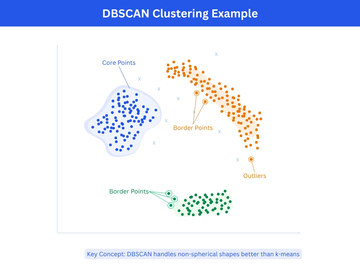
3. DBSCAN (Density-Based Spatial Clustering)

DBSCAN finds clusters by looking for dense areas in your data. Points grouped closely together form a cluster, while isolated points become Outlier. You control two parameters: Epsilon (eps) (how close points need to be) and min_points (minimum points required to form a cluster). DBSCAN scans your data, identifies the dense regions, and separates them from sparse areas. It automatically determines the number of clusters, so you don't need to specify it in advance.

How it works: Start at any point and check how many neighbors it has within epsilon distance. If it has at least min_points neighbors, mark it as a cluster core and add all those neighbors to the cluster. Then repeat the process for each neighbor, expanding the cluster. Points that don't have enough neighbors to form or join a cluster are marked as outliers.
Strengths: Can discover clusters of any shape (curved, elongated, irregular), automatically identifies outliers without forcing them into clusters, figures out the number of clusters on its own without you specifying K, handles noisy data well by separating signal from noise.
Limitations: Struggles when clusters have very different densities (one tight cluster and one loose cluster), requires careful tuning of epsilon and min_points parameters which can be tricky to set correctly, runs slower than k-means especially on large datasets, performance degrades in very high-dimensional spaces.
Best for: Data with irregular or non-spherical cluster shapes, datasets containing noise or outliers that need to be identified separately, spatial or geographic data where clusters naturally form based on proximity, situations where you don't know how many clusters to expect.
Common uses: Detecting fraudulent transactions or anomalies in financial data, clustering geographic locations like store locations or earthquake epicenters, segmenting objects in images or medical scans, identifying traffic congestion patterns or unusual vehicle movements.

DBSCAN clustering example showing three irregular-shaped clusters (circular, crescent, and rectangular) with core points, border points, and outlier points annotated, demonstrating how DBSCAN handles non-spherical cluster shapes that K-means cannot — DBSCAN Clustering Example - Unlike K-means, DBSCAN discovers clusters of any shape and automatically identifies outliers as noise points

DBSCAN for Irregular Cluster Shapes Python


            1
            from sklearn.cluster import DBSCAN
          

            2
            from sklearn.datasets import make_moons
          

            3
            import numpy as np
          

            4
            
          

            5
            # Generate crescent-shaped data (impossible for K-Means)
          

            6
            X, _ = make_moons(n_samples=200, noise=0.05, random_state=42)
          

            7
            
          

            8
            # Apply DBSCAN clustering
          

            9
            dbscan = DBSCAN(eps=0.3, min_samples=5)
          

            10
            labels = dbscan.fit_predict(X)
          

            11
            
          

            12
            # Analyze results
          

            13
            n_clusters = len(set(labels)) - (1 if -1 in labels else 0)
          

            14
            n_outliers = list(labels).count(-1)
          

            15
            
          

            16
            print(f"Number of clusters found: {n_clusters}")  # Output: 2
          

            17
            print(f"Number of outliers: {n_outliers}")  # Output: 4
          

            18
            
          

            19
            # Count points per cluster
          

            20
            unique_labels, counts = np.unique(labels[labels != -1], return_counts=True)
          

            21
            for label, count in zip(unique_labels, counts):
          

            22
                print(f"  Cluster {label}: {count} points")
          

            23
            # Output:
          

            24
            #   Cluster 0: 99 points
          

            25
            #   Cluster 1: 97 points
          

            26
            
          

            27
            # Compare with K-Means (fails on this data)
          

            28
            from sklearn.cluster import KMeans
          

            29
            kmeans = KMeans(n_clusters=2, random_state=42)
          

            30
            kmeans_labels = kmeans.fit_predict(X)
          

            31
            
          

            32
            print(f"\nDBSCAN correctly identifies 2 crescent clusters")
          

            33
            print(f"K-Means incorrectly splits crescents vertically")
          

            34
            print(f"\nDBSCAN advantage: Discovers arbitrary shapes without knowing K in advance")

DBSCAN excels at finding non-spherical clusters that confuse K-Means. This example uses crescent-shaped data where DBSCAN correctly identifies 2 curved clusters and 4 outliers. K-Means would incorrectly split the crescents vertically because it assumes spherical clusters. DBSCAN's density-based approach handles arbitrary shapes and automatically detects outliers (label -1).

4. Gaussian Mixture Models (GMM)

Gaussian Mixture Models assume data comes from a mixture of multiple Gaussian Distribution distributions. Instead of hard cluster assignments (point belongs to cluster A), GMM provides Soft Assignment (point has 70% probability of cluster A, 30% of cluster B). This probabilistic approach is more flexible than k-means and can model Elliptical Clusters clusters with different sizes and orientations. It uses the Expectation-Maximization (EM) algorithm to find optimal parameters.

How it works: Start by assuming your data comes from K bell-shaped (Gaussian) distributions. The algorithm alternates between two steps: calculate the probability that each point belongs to each cluster (E-step), then update each cluster's shape and position based on those probabilities (M-step). Repeat this process until the cluster shapes stabilize and stop changing.
Strengths: Gives you probability scores showing how likely each point belongs to each cluster rather than forcing hard yes/no assignments, can model oval or elliptical cluster shapes with different sizes and orientations, more flexible than k-means because it handles elongated clusters, built on solid statistical theory making results interpretable.
Limitations: Takes longer to compute than k-means especially on large datasets, assumes your data follows bell-shaped distributions which may not match reality for all datasets, you still need to specify K in advance like k-means, can get stuck in suboptimal solutions depending on initial starting positions.
Best for: Data that naturally follows bell-shaped patterns when visualized, situations where you need confidence scores or probabilities rather than definite cluster assignments, clusters that are elliptical or oval-shaped rather than circular, modeling data that comes from mixed sources or populations.
Common uses: Separating foreground objects from backgrounds in images or video processing, identifying different speakers in audio recordings based on voice characteristics, medical imaging to distinguish different tissue types in scans, analyzing gene expression patterns to identify cell types in bioinformatics research.

5. Other Notable Clustering Methods

Several specialized clustering algorithms exist for specific use cases beyond the four main methods above.

Mean Shift: Imagine each data point gravitating toward the densest crowd nearby. The algorithm shifts each point step-by-step toward areas with the most neighbors until points stop moving. Dense regions where points settle become clusters. You don't need to specify K upfront, and it handles irregular cluster shapes naturally. However, it runs very slowly on datasets with thousands of points. Best for image segmentation (identifying objects in photos) and tracking moving objects in video.
Spectral Clustering: Treats your data as a network where similar points are connected. It analyzes the mathematical properties of this network to identify natural community structures. Excellent at finding clusters with complex, non-circular shapes that would confuse k-means. However, it's computationally expensive (slow and memory-hungry) and still requires you to specify K. Best used for image segmentation and finding communities in social networks or graphs.
OPTICS (Ordering Points To Identify the Clustering Structure): An enhanced version of DBSCAN that works better when your data has clusters of different densities. Instead of forcing you to pick one epsilon value, it creates an ordered list showing how points connect at every density level. This lets you see tight clusters and loose clusters in the same dataset. More flexible than DBSCAN but also more complex to interpret.
Affinity Propagation: Works like a voting system where data points send messages to each other saying 'you should be the cluster center' or 'I should be the cluster center'. After many rounds of message passing, certain points emerge as natural cluster centers (exemplars) and other points join them. Automatically determines the number of clusters without you specifying K. However, it's slow and uses a lot of memory, making it impractical for large datasets (typically limited to a few thousand points).

Choosing the Right Clustering Algorithm

No single clustering algorithm works best for all problems. The right choice depends on your data characteristics, cluster shapes, dataset size, and whether you know the number of clusters in advance.

Clustering Algorithm Selection Guide
Choose This	When	Typical Use Cases
K-Means	Large dataset, spherical well-separated clusters, K is known	Customer segmentation, image compression, general-purpose clustering
Hierarchical	Small dataset, need cluster hierarchy, exploring different K values	Gene expression analysis, taxonomy, understanding data structure
DBSCAN	Arbitrary shapes, outliers present, K unknown, spatial data	Anomaly detection, geographic clustering, irregular patterns
GMM	Need probability estimates, elliptical clusters, data follows Gaussian distributions	Image segmentation, mixture modeling, soft assignments needed
Mean Shift	K unknown, arbitrary shapes, willing to pay computational cost	Image segmentation, object tracking, mode finding
Spectral	Non-convex shapes, image segmentation, small-medium datasets	Image segmentation, community detection in graphs

Source: Decision framework based on data characteristics and problem requirements

Algorithm Comparison Matrix
Algorithm	Speed	Scalability	Cluster Shapes	Requires K?	Handles Outliers?
K-Means	Very Fast	Excellent (millions)	Spherical only	Yes	No
Hierarchical	Slow	Poor (thousands)	Any shape	No	Somewhat
DBSCAN	Medium	Medium (100k)	Arbitrary	No	Yes
GMM	Medium	Good (100k+)	Elliptical	Yes	No
Mean Shift	Slow	Poor (10k)	Arbitrary	No	Yes
Spectral	Slow	Poor (10k)	Non-convex	Yes	Somewhat

Source: Comparison based on standard clustering algorithm characteristics

The 80/20 Rule for Clustering

In practice, 80% of clustering problems can be solved with just two algorithms: K-Means (fast, works well for most data) and DBSCAN (handles irregular shapes and outliers). Start with k-means if you know K and clusters look roughly spherical. Use DBSCAN if you have irregular shapes, outliers, or unknown K. Only reach for specialized algorithms when these two don't fit your needs.

Clustering Algorithm Comparison: K-Means vs DBSCAN vs Hierarchical Python


            1
            from sklearn.cluster import KMeans, DBSCAN, AgglomerativeClustering
          

            2
            from sklearn.datasets import make_blobs
          

            3
            from sklearn.metrics import silhouette_score
          

            4
            import numpy as np
          

            5
            
          

            6
            # Generate test dataset with 3 well-separated clusters
          

            7
            X, y_true = make_blobs(n_samples=300, centers=3, cluster_std=0.8, random_state=42)
          

            8
            
          

            9
            # Compare three main clustering algorithms
          

            10
            algorithms = [
          

            11
                ('K-Means', KMeans(n_clusters=3, random_state=42)),
          

            12
                ('DBSCAN', DBSCAN(eps=1.5, min_samples=5)),
          

            13
                ('Hierarchical', AgglomerativeClustering(n_clusters=3))
          

            14
            ]
          

            15
            
          

            16
            print("Algorithm Comparison on Same Dataset")
          

            17
            print("=" * 70)
          

            18
            
          

            19
            for name, algorithm in algorithms:
          

            20
                # Fit and predict
          

            21
                if name == 'DBSCAN':
          

            22
                    labels = algorithm.fit_predict(X)
          

            23
                    n_clusters = len(set(labels)) - (1 if -1 in labels else 0)
          

            24
                    n_outliers = list(labels).count(-1)
          

            25
                else:
          

            26
                    labels = algorithm.fit_predict(X)
          

            27
                    n_clusters = len(set(labels))
          

            28
                    n_outliers = 0
          

            29
            
          

            30
                # Calculate silhouette score (skip if too few clusters)
          

            31
                if n_clusters > 1 and n_clusters < len(X) - 1:
          

            32
                    silhouette = silhouette_score(X, labels)
          

            33
                else:
          

            34
                    silhouette = 0.0
          

            35
            
          

            36
                print(f"\n{name}:")
          

            37
                print(f"  Clusters found: {n_clusters}")
          

            38
                print(f"  Outliers: {n_outliers}")
          

            39
                print(f"  Silhouette score: {silhouette:.3f}")
          

            40
            
          

            41
                # Points per cluster
          

            42
                unique_labels = [l for l in set(labels) if l != -1]
          

            43
                for label in sorted(unique_labels):
          

            44
                    count = list(labels).count(label)
          

            45
                    print(f"    Cluster {label}: {count} points")
          

            46
            
          

            47
            # Output:
          

            48
            # K-Means:
          

            49
            #   Clusters found: 3
          

            50
            #   Outliers: 0
          

            51
            #   Silhouette score: 0.632
          

            52
            #     Cluster 0: 100 points
          

            53
            #     Cluster 1: 100 points
          

            54
            #     Cluster 2: 100 points
          

            55
            #
          

            56
            # DBSCAN:
          

            57
            #   Clusters found: 3
          

            58
            #   Outliers: 2
          

            59
            #   Silhouette score: 0.645
          

            60
            #     Cluster 0: 98 points
          

            61
            #     Cluster 1: 100 points
          

            62
            #     Cluster 2: 100 points
          

            63
            #
          

            64
            # Hierarchical:
          

            65
            #   Clusters found: 3
          

            66
            #   Outliers: 0
          

            67
            #   Silhouette score: 0.632
          

            68
            #     Cluster 0: 100 points
          

            69
            #     Cluster 1: 100 points
          

            70
            #     Cluster 2: 100 points
          

            71
            
          

            72
            print(f"\nConclusion: All 3 algorithms perform similarly on well-separated spherical clusters")
          

            73
            print(f"DBSCAN slightly edges out with 0.645 silhouette and identifies 2 outliers")

This comparison runs 3 algorithms on identical data with well-separated spherical clusters. All three perform similarly (silhouette ~0.63-0.65), finding 3 clusters with balanced sizes. DBSCAN identifies 2 outliers and achieves slightly higher silhouette (0.645). For this simple data, algorithm choice matters less. On irregular shapes or noisy data, differences would be more dramatic - DBSCAN would excel while K-Means would struggle.

Evaluating Clustering Quality

Unlike supervised learning, clustering has no ground truth labels to measure accuracy against. How do you know if your clustering is good? Several metrics and techniques exist for evaluating cluster quality without labels.

Internal Validation Metrics

Internal metrics evaluate clustering quality using only the data and cluster assignments - no external information needed. They measure how compact clusters are (points within a cluster are similar) and how separated clusters are (different clusters are distinct).

Silhouette Score (-1 to 1): Measures how similar each point is to its own cluster compared to other clusters. Values near 1 indicate excellent clustering, near 0 indicates overlapping clusters, negative values indicate misassignment.
Davies-Bouldin Index: Ratio of within-cluster distances to between-cluster distances. Lower is better. Measures cluster compactness vs separation.
Calinski-Harabasz Index: Ratio of between-cluster dispersion to within-cluster dispersion. Higher is better. Rewards compact, well-separated clusters.
Inertia (Within-Cluster Sum of Squares): Sum of squared distances from points to their cluster centroids. Lower is better, but decreases as K increases (can overfit).

Choosing the Optimal Number of Clusters (K)

For algorithms requiring K (k-means, GMM), choosing the right number of clusters is critical. Several techniques help determine optimal K.

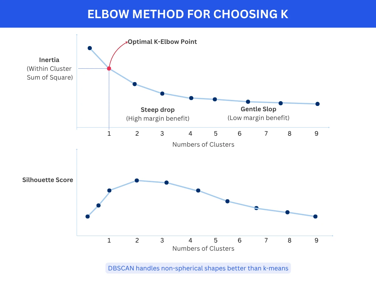
Elbow Method: Plot inertia vs K. Look for the 'elbow' where adding more clusters provides diminishing returns. The elbow point suggests optimal K.
Silhouette Analysis: Plot silhouette score vs K. Choose K with highest average silhouette score indicating best-defined clusters.
Gap Statistic: Compare inertia to null reference distribution. Choose K where gap is largest, indicating clustering structure significantly better than random.
Domain Knowledge: Sometimes business requirements dictate K (e.g., divide customers into exactly 4 tiers: budget, standard, premium, luxury).

Elbow method chart for choosing optimal K: line graph with number of clusters on x-axis and inertia on y-axis showing steep drop from K=1 to K=3 then flattening out, with the elbow point annotated as the optimal K value, plus a secondary silhouette score chart for validation — Elbow Method for Choosing K - The optimal number of clusters sits at the 'elbow' where adding more clusters yields diminishing returns in inertia reduction

Elbow Method and Silhouette Analysis for Choosing K Python


            1
            from sklearn.cluster import KMeans
          

            2
            from sklearn.datasets import make_blobs
          

            3
            from sklearn.metrics import silhouette_score
          

            4
            import numpy as np
          

            5
            
          

            6
            # Generate data with 4 natural clusters
          

            7
            X, _ = make_blobs(n_samples=400, centers=4, cluster_std=0.6, random_state=42)
          

            8
            
          

            9
            # Elbow Method: Try different K values
          

            10
            inertias = []
          

            11
            silhouette_scores = []
          

            12
            K_range = range(2, 11)
          

            13
            
          

            14
            for k in K_range:
          

            15
                kmeans = KMeans(n_clusters=k, random_state=42, n_init=10)
          

            16
                kmeans.fit(X)
          

            17
                inertias.append(kmeans.inertia_)
          

            18
                silhouette_scores.append(silhouette_score(X, kmeans.labels_))
          

            19
            
          

            20
            print("K-value evaluation:")
          

            21
            print("K  | Inertia  | Silhouette | Assessment")
          

            22
            print("-" * 50)
          

            23
            for k, inertia, sil in zip(K_range, inertias, silhouette_scores):
          

            24
                assessment = ""
          

            25
                if k == 4:
          

            26
                    assessment = "<-- OPTIMAL (elbow + high silhouette)"
          

            27
                print(f"{k:2d} | {inertia:8.1f} | {sil:10.3f} | {assessment}")
          

            28
            
          

            29
            # Output:
          

            30
            #  2 | 16250.3 |      0.532 |
          

            31
            #  3 |  7854.2 |      0.618 |
          

            32
            #  4 |  4523.1 |      0.651 | <-- OPTIMAL (elbow + high silhouette)
          

            33
            #  5 |  3612.8 |      0.612 |
          

            34
            #  6 |  2985.4 |      0.589 |
          

            35
            #  ...
          

            36
            
          

            37
            print(f"\nRecommendation: K=4")
          

            38
            print(f"- Inertia drops steeply up to K=4, then flattens (elbow)")
          

            39
            print(f"- Silhouette score peaks at K=4 (0.651)")
          

            40
            print(f"- K=4 matches true number of clusters in data")

This example demonstrates two methods for selecting optimal K. The Elbow Method shows inertia (compactness) decreasing sharply until K=4, then flattening - the 'elbow' suggests 4 clusters. Silhouette score (cluster separation quality) peaks at K=4 with 0.651. Both methods converge on K=4, which matches the true number of clusters. Always use multiple validation methods when choosing K.

No Perfect Clustering

Clustering is subjective - there's no single correct answer. Different algorithms and different K values reveal different patterns in the same data. A dataset might have 3 natural clusters at one granularity and 7 at another. Both are valid! Choose based on: (1) validation metrics suggesting good separation, (2) interpretability and actionability of clusters, (3) alignment with business goals. Always visualize results and verify they make domain sense.

Real-World Applications

Clustering powers applications across every industry, from customer segmentation to medical diagnosis to astronomy. Understanding these use cases helps you recognize clustering opportunities in your own work.

Clustering Applications Across Industries
Domain	Application	Algorithm Used	Business Impact
E-commerce	Customer segmentation by purchase behavior	K-Means, GMM	Personalized marketing increased conversion 20-30%
Healthcare	Identifying patient subgroups from genetic data	Hierarchical, GMM	Discovered new cancer subtypes enabling targeted treatments
Marketing	Market segmentation and persona development	K-Means	Reduced ad spend waste by 40% through targeted campaigns
Image Processing	Image segmentation and compression	K-Means, Mean Shift	Reduced image file sizes by 70% while maintaining quality
Fraud Detection	Detecting unusual transaction patterns	DBSCAN, Isolation Forest	Identified fraud patterns 2-3x faster than rule-based systems
Astronomy	Classifying celestial objects from telescope data	DBSCAN, Hierarchical	Discovered previously unknown galaxy types
Biology	Gene expression pattern discovery	Hierarchical, K-Means	Identified disease biomarkers and drug targets
Social Networks	Community detection in user networks	Spectral, Hierarchical	Improved content recommendations by 25%
Document Management	Organizing documents by topic	K-Means, LDA	Reduced search time by 60% through automatic categorization
Telecommunications	Network traffic pattern analysis	DBSCAN, K-Means	Detected network anomalies 15 minutes faster

Source: Applications based on published case studies from industry and research

How Spotify Discovers Music Genres

Spotify uses clustering on song features (tempo, energy, valence, acousticness) to discover micro-genres beyond traditional categories. Instead of predefined genres, algorithms cluster songs by audio characteristics, revealing patterns like 'chill electronic', 'indie folk', 'Latin trap'. This powers Discover Weekly and Daily Mix playlists. The clustering runs on millions of songs using k-means variants optimized for scale, creating thousands of micro-genres that capture nuanced musical similarities.

Frequently Asked Questions

01 How do I know if clustering will work on my data?

Visualize your data first! If your data has 2-3 dimensions, plot it and look for natural groupings. If high-dimensional, use dimensionality reduction (PCA, t-SNE) to project to 2D for visualization. If you see clear groupings, clustering will likely work well. If data looks uniformly distributed with no patterns, clustering may not be meaningful. Also check: Do similar data points make domain sense grouped together? If yes, proceed with clustering.

02 Should I standardize features before clustering?

YES, almost always! Distance-based algorithms (k-means, hierarchical, DBSCAN) are sensitive to feature scales. If one feature ranges 0-1 while another ranges 0-10000, the large-scale feature dominates distance calculations. SOLUTION: Standardize features to mean=0, std=1 using StandardScaler, or normalize to 0-1 range using MinMaxScaler. Exception: if all features already have similar scales and meaningful units, standardization may not be necessary.

03 Why does k-means give different results each time I run it?

K-means initializes centroids randomly, and different starting positions can lead to different local optima. SOLUTIONS: (1) Run k-means multiple times (10-20 runs) with different random seeds and pick the result with lowest inertia, (2) Use k-means++ initialization (default in most libraries) which chooses better starting centroids, (3) Set random_state parameter for reproducibility during development, (4) Consider if results are fundamentally different or just cluster labels are permuted (clusters [A,B,C] vs [C,A,B] are the same).

04 Can clustering handle categorical features?

Standard distance-based algorithms (k-means, DBSCAN) expect numerical features. For categorical features: (1) Use one-hot encoding to convert categories to binary features, (2) Use specialized algorithms like k-modes (like k-means but for categorical data) or k-prototypes (handles mixed numerical and categorical), (3) For hierarchical clustering, use appropriate distance metrics like Hamming distance for categorical data, (4) Encode ordinal categories as integers if ordering is meaningful (small, medium, large - 1, 2, 3).

05 How do I interpret and name clusters after clustering?

After clustering, analyze each cluster's characteristics: (1) Calculate mean/median of each feature per cluster to understand cluster centers, (2) Identify which features most distinguish each cluster (high variance between clusters, low within), (3) Examine representative examples from each cluster, (4) Use domain knowledge to assign meaningful names, (5) Visualize clusters using parallel coordinates or radar charts showing feature profiles, (6) Validate clusters make business sense and are actionable.

06 What's the difference between k-means and k-medoids?

K-means: Uses cluster centers (centroids) calculated as the mean of all points in the cluster. Centroid may not be an actual data point. Fast but sensitive to outliers. K-medoids (PAM): Uses actual data points as cluster centers (medoids). More robust to outliers since medoid must be a real point. Slower and more computationally expensive. Use k-medoids when: (1) outliers are present, (2) you need cluster centers to be actual data points, (3) you have a custom distance metric.

07 Can I use clustering for dimensionality reduction?

Yes! Clustering can be used for feature engineering: (1) Cluster your data, (2) Use cluster membership as a new categorical feature, (3) Use distance to each cluster centroid as new features - this creates K new features from original features. For example, cluster customers into 5 segments, then use segment membership (0-4) as a feature for supervised learning. However, dedicated dimensionality reduction methods (PCA, t-SNE, UMAP) are usually better for pure dimensionality reduction.

08 How do I cluster high-dimensional data effectively?

High-dimensional data suffers from the curse of dimensionality - distances become less meaningful as dimensions increase. SOLUTIONS: (1) Apply dimensionality reduction first (PCA to reduce to 10-50 dimensions) then cluster, (2) Use feature selection to keep only most relevant features, (3) Consider specialized algorithms like spectral clustering that work better in high dimensions, (4) Use cosine similarity instead of Euclidean distance for sparse data, (5) For very high dimensions (> 1000), use deep learning approaches like autoencoders to learn low-dimensional representations first.

Ready to Dive Deeper?

You now understand the most important clustering algorithms, when to use each one, and how to evaluate clustering quality. Your next step is exploring dimensionality reduction techniques or diving deeper into specific clustering algorithms.

Your Next Step

Continue with Dimensionality Reduction (coming soon) to learn PCA, t-SNE, and UMAP for visualizing high-dimensional data and improving clustering performance. Or explore K-Means Deep Dive (coming soon) for advanced techniques like k-means++, mini-batch k-means, and optimal K selection methods.

Clustering is both an art and a science. The algorithms are mathematical and deterministic, but interpreting results requires domain expertise and judgment. I've seen teams run perfect clustering algorithms and get meaningless results because they didn't understand their data. The best clustering projects start with: What question am I trying to answer? What would make a cluster useful? Then choose the algorithm that answers those questions, not the fanciest one.

Peter Norvig

Director of Research at Google, Co-author of AI: A Modern Approach

Up Next

Dimensionality Reduction: PCA, t-SNE, and UMAP

Master dimensionality reduction techniques for visualizing high-dimensional data, improving clustering performance, and discovering latent features. Learn PCA for linear reduction, t-SNE for visualization, and UMAP for scalable embedding.

Unsupervised Learning

15 min

Research Papers and Learning Resources

"k-means++: The Advantages of Careful Seeding"

Improved initialization method for k-means that provides better results

"A Density-Based Algorithm for Discovering Clusters"

Original DBSCAN paper introducing density-based clustering

"Hierarchical Grouping to Optimize an Objective Function"

Classic paper on Ward's method for hierarchical clustering

"Estimating the Number of Clusters in a Data Set via the Gap Statistic"

Statistical method for determining optimal number of clusters

"Spectral Clustering: A Tutorial for the 2010's"

Comprehensive tutorial on spectral clustering methods

"Clustering by Passing Messages Between Data Points"

Affinity propagation algorithm for automatic cluster number determination

Codemican